R ggplot2 geom_violin 小提琴情节

geom_violin(
  mapping = NULL,
  data = NULL,
  stat = "ydensity",
  position = "dodge",
  ...,
  draw_quantiles = NULL,
  trim = TRUE,
  scale = "area",
  na.rm = FALSE,
  orientation = NA,
  show.legend = NA,
  inherit.aes = TRUE
)

stat_ydensity(
  mapping = NULL,
  data = NULL,
  geom = "violin",
  position = "dodge",
  ...,
  bw = "nrd0",
  adjust = 1,
  kernel = "gaussian",
  trim = TRUE,
  scale = "area",
  na.rm = FALSE,
  orientation = NA,
  show.legend = NA,
  inherit.aes = TRUE
)

geom_violin() 为示例，stat_density() 为沿 x 轴的数据示例。

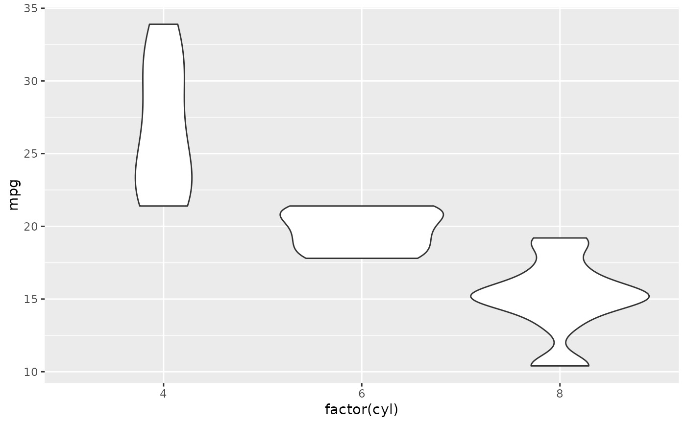
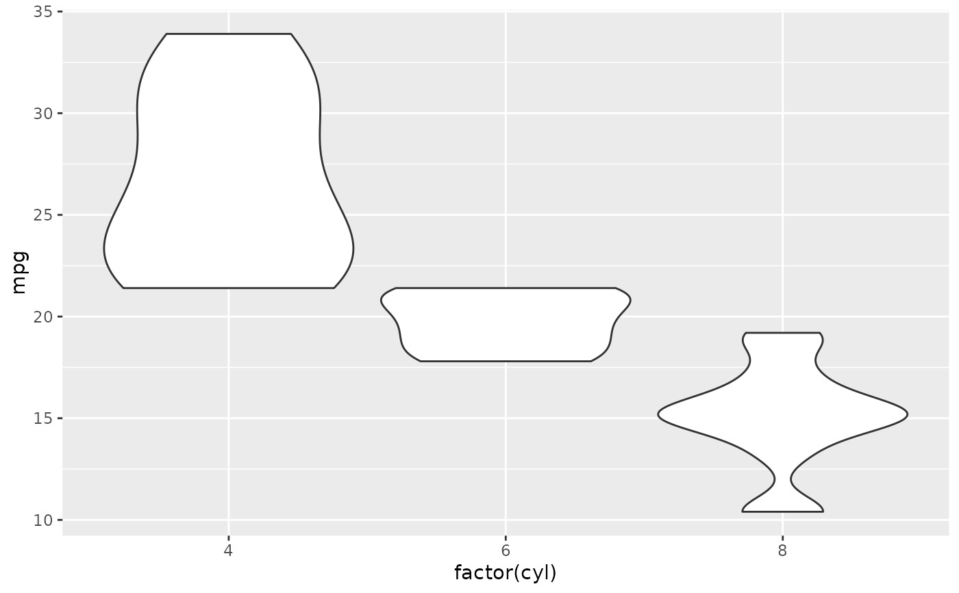
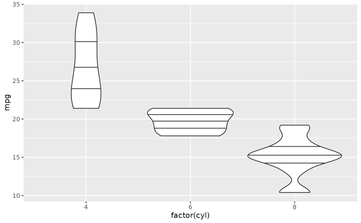
p <- ggplot(mtcars, aes(factor(cyl), mpg))
p + geom_violin()


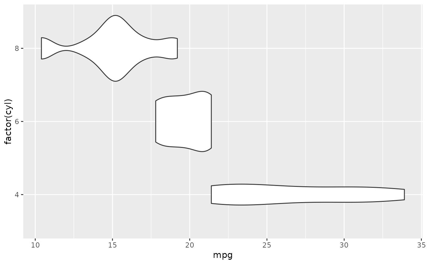
# Orientation follows the discrete axis
ggplot(mtcars, aes(mpg, factor(cyl))) +
  geom_violin()


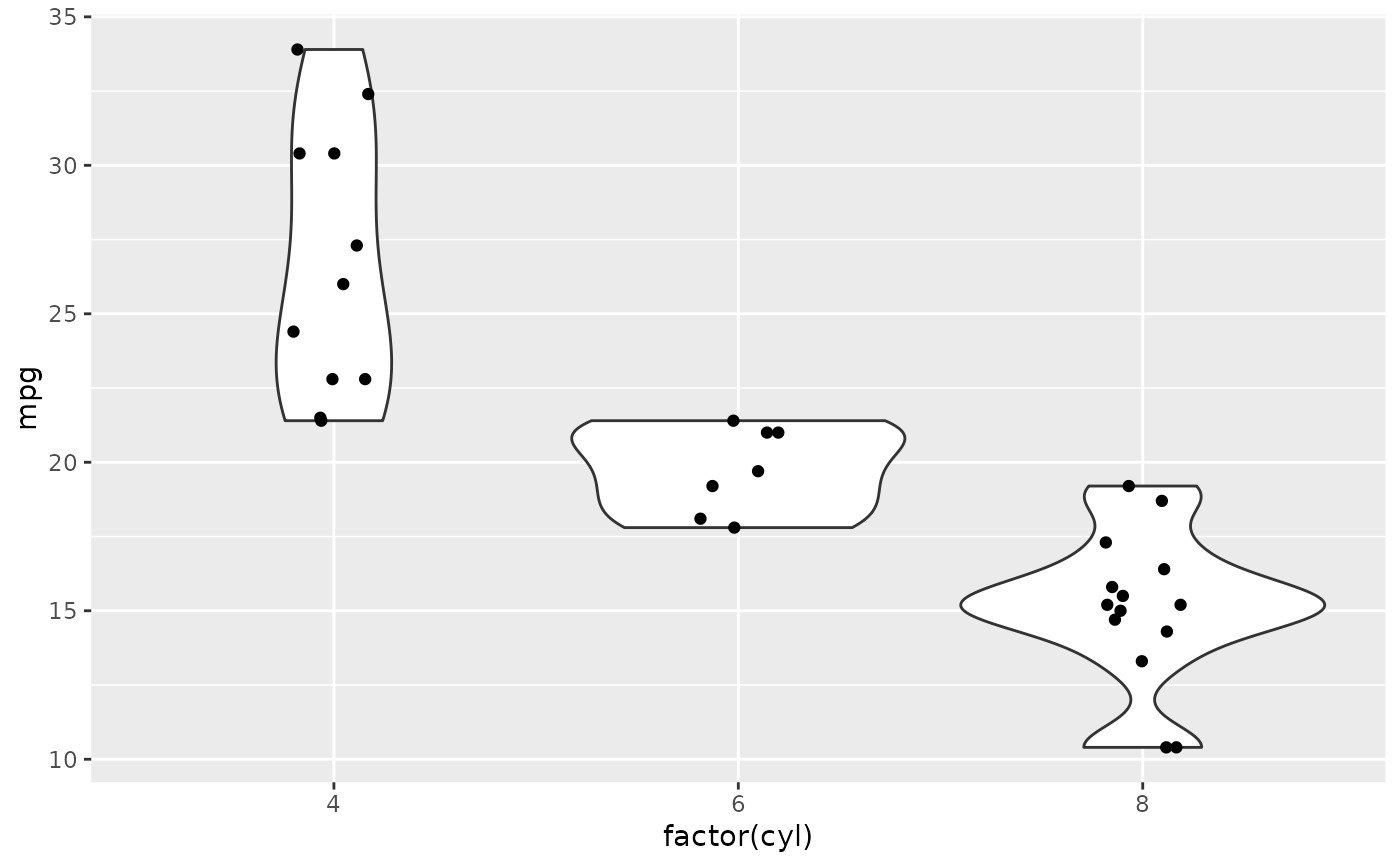
# \donttest{
p + geom_violin() + geom_jitter(height = 0, width = 0.1)


# Scale maximum width proportional to sample size:
p + geom_violin(scale = "count")


# Scale maximum width to 1 for all violins:
p + geom_violin(scale = "width")


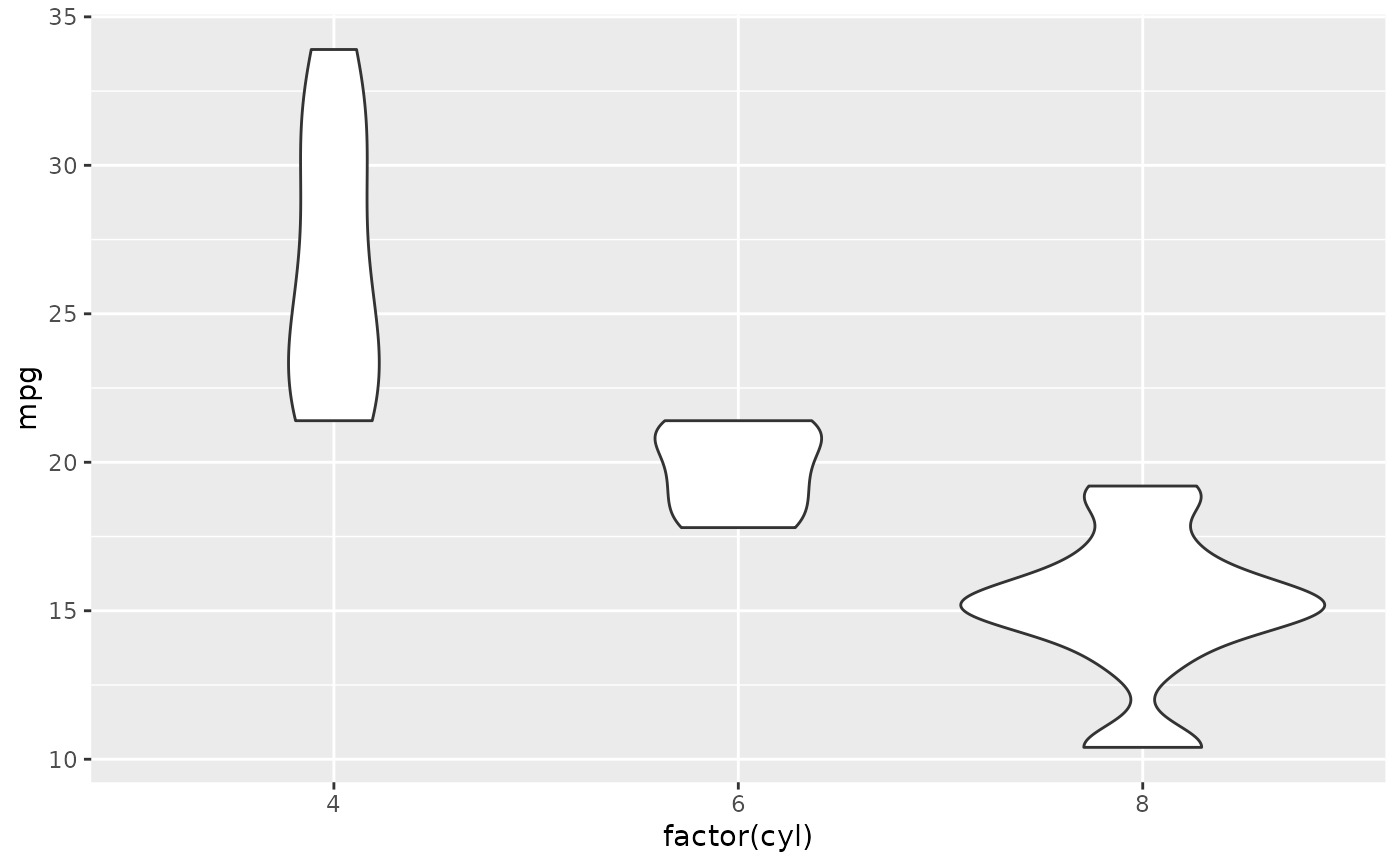
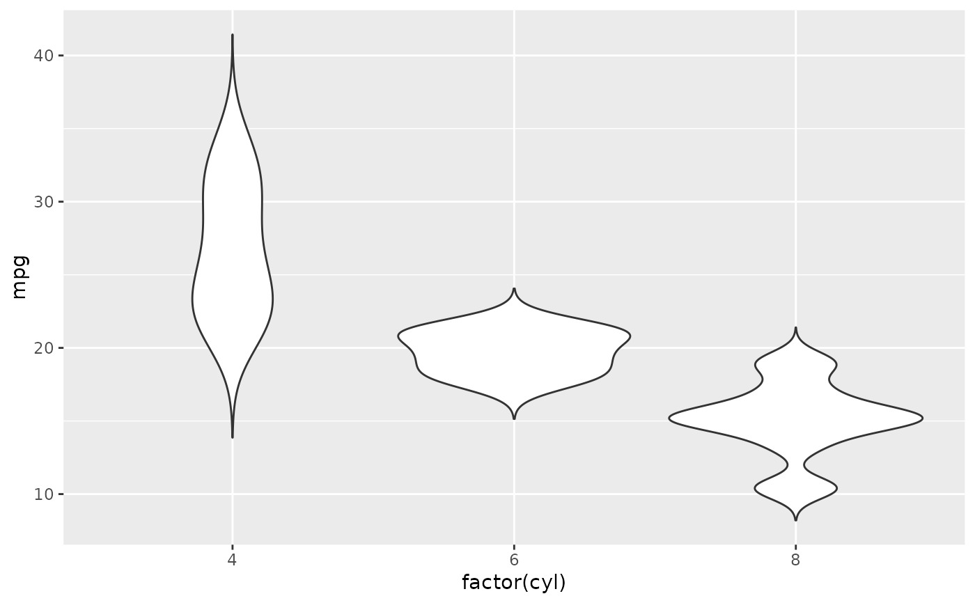
# Default is to trim violins to the range of the data. To disable:
p + geom_violin(trim = FALSE)


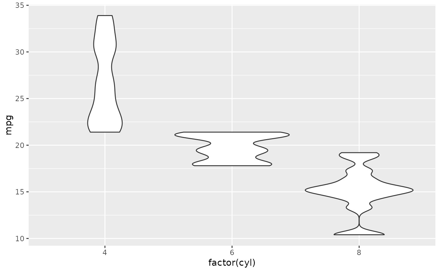
# Use a smaller bandwidth for closer density fit (default is 1).
p + geom_violin(adjust = .5)


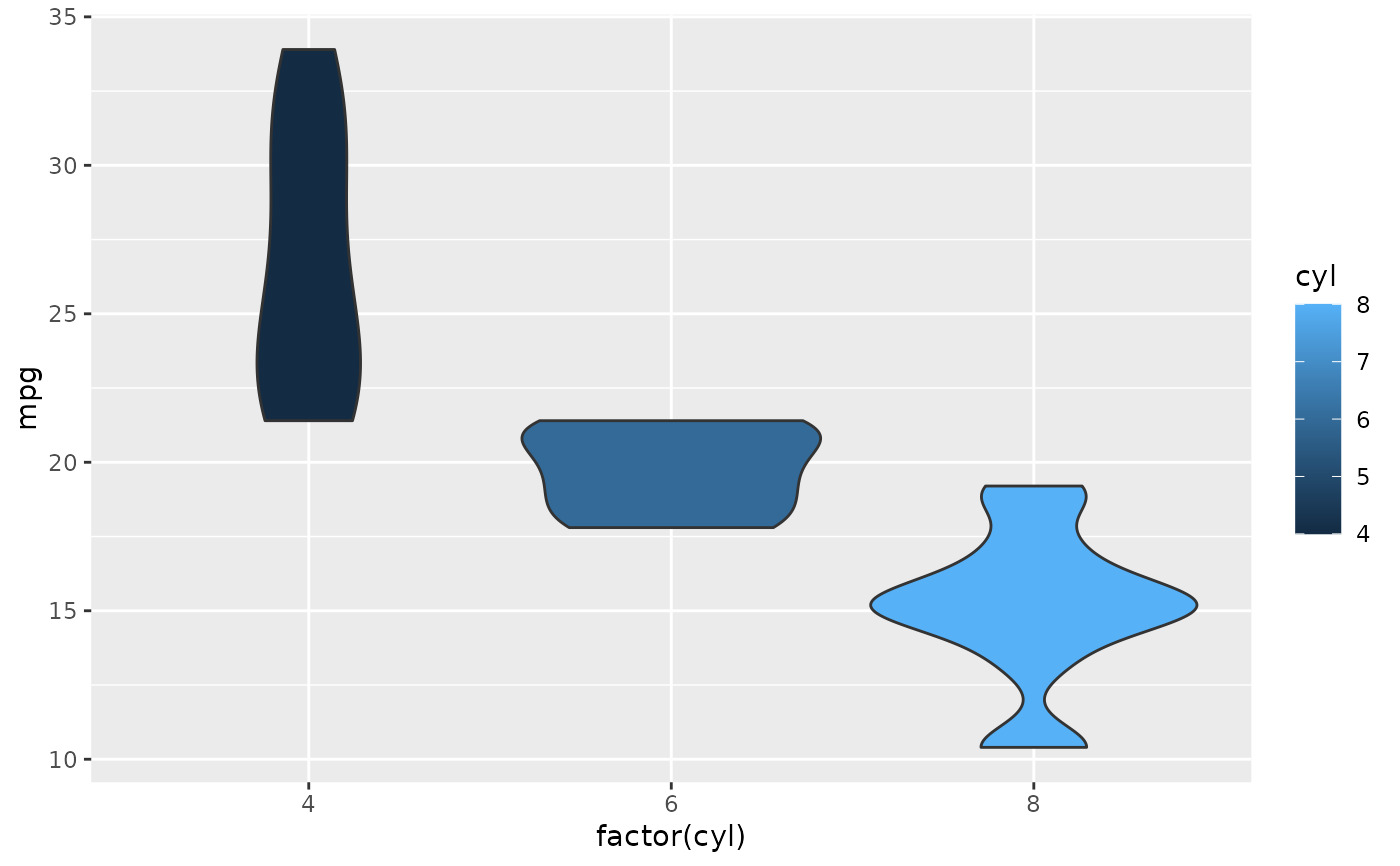
# Add aesthetic mappings
# Note that violins are automatically dodged when any aesthetic is
# a factor
p + geom_violin(aes(fill = cyl))

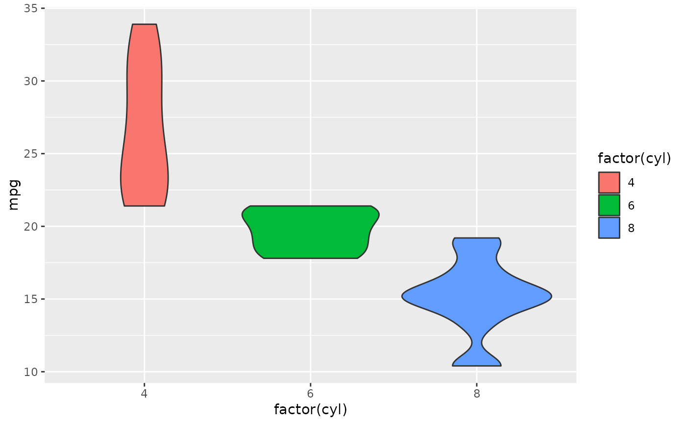
p + geom_violin(aes(fill = factor(cyl)))

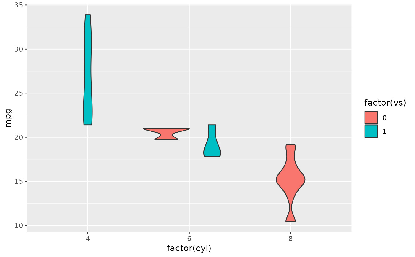
p + geom_violin(aes(fill = factor(vs)))
#> Warning: Groups with fewer than two data points have been dropped.

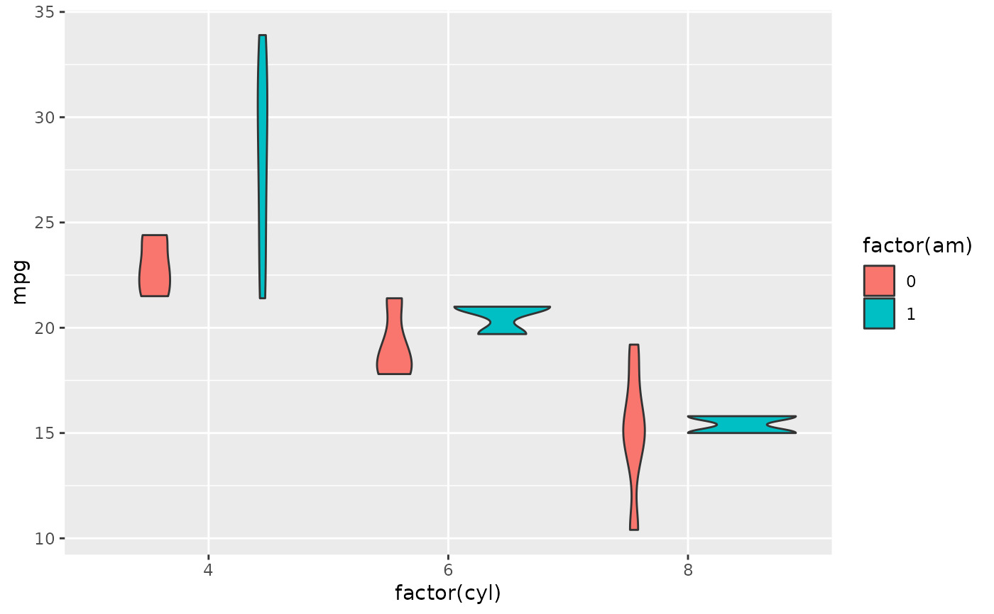
p + geom_violin(aes(fill = factor(am)))


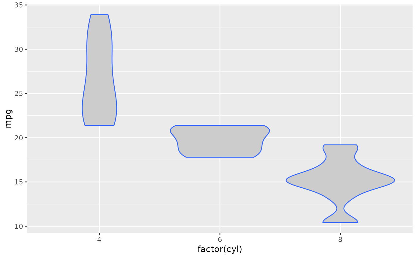
# Set aesthetics to fixed value
p + geom_violin(fill = "grey80", colour = "#3366FF")


# Show quartiles
p + geom_violin(draw_quantiles = c(0.25, 0.5, 0.75))


# Scales vs. coordinate transforms -------
if (require("ggplot2movies")) {
# Scale transformations occur before the density statistics are computed.
# Coordinate transformations occur afterwards.  Observe the effect on the
# number of outliers.
m <- ggplot(movies, aes(y = votes, x = rating, group = cut_width(rating, 0.5)))
m + geom_violin()
m +
  geom_violin() +
  scale_y_log10()
m +
  geom_violin() +
  coord_trans(y = "log10")
m +
  geom_violin() +
  scale_y_log10() + coord_trans(y = "log10")

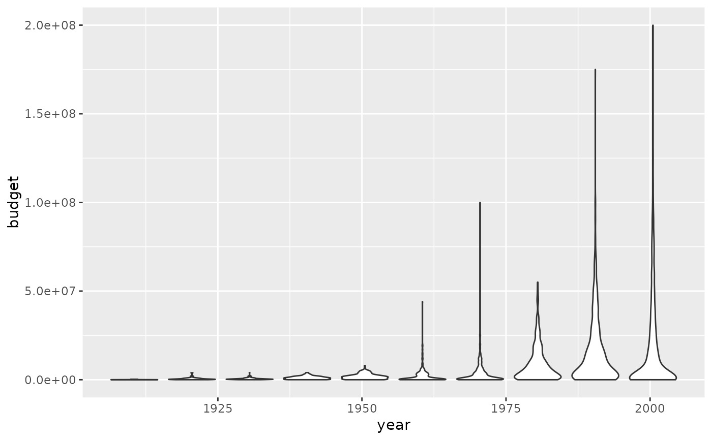
# Violin plots with continuous x:
# Use the group aesthetic to group observations in violins
ggplot(movies, aes(year, budget)) +
  geom_violin()
ggplot(movies, aes(year, budget)) +
  geom_violin(aes(group = cut_width(year, 10)), scale = "width")
}
#> Warning: Removed 53573 rows containing non-finite values (`stat_ydensity()`).
#> Warning: Groups with fewer than two data points have been dropped.

# }