通过将 x 轴划分为多个箱并计算每个箱中的观测值数量,可视化单个连续变量的分布。直方图 (geom_histogram()) 用条形显示计数;频率多边形 (geom_freqpoly()) 用线条显示计数。当您想要比较分类变量各个级别的分布时,频率多边形更合适。
用法
geom_freqpoly(
  mapping = NULL,
  data = NULL,
  stat = "bin",
  position = "identity",
  ...,
  na.rm = FALSE,
  show.legend = NA,
  inherit.aes = TRUE
)

geom_histogram(
  mapping = NULL,
  data = NULL,
  stat = "bin",
  position = "stack",
  ...,
  binwidth = NULL,
  bins = NULL,
  na.rm = FALSE,
  orientation = NA,
  show.legend = NA,
  inherit.aes = TRUE
)

stat_bin(
  mapping = NULL,
  data = NULL,
  geom = "bar",
  position = "stack",
  ...,
  binwidth = NULL,
  bins = NULL,
  center = NULL,
  boundary = NULL,
  breaks = NULL,
  closed = c("right", "left"),
  pad = FALSE,
  na.rm = FALSE,
  orientation = NA,
  show.legend = NA,
  inherit.aes = TRUE
)
参数
- mapping
-
由
aes()创建的一组美学映射。如果指定且inherit.aes = TRUE(默认),它将与绘图顶层的默认映射组合。如果没有绘图映射,则必须提供mapping。 - data
-
该层要显示的数据。有以下三种选择:
如果默认为
NULL,则数据继承自ggplot()调用中指定的绘图数据。data.frame或其他对象将覆盖绘图数据。所有对象都将被强化以生成 DataFrame 。请参阅fortify()将为其创建变量。将使用单个参数(绘图数据)调用
function。返回值必须是data.frame,并将用作图层数据。可以从formula创建function(例如~ head(.x, 10))。 - position
-
位置调整,可以是命名调整的字符串(例如
"jitter"使用position_jitter),也可以是调用位置调整函数的结果。如果需要更改调整设置,请使用后者。 - ...
-
其他参数传递给
layer()。这些通常是美学,用于将美学设置为固定值,例如colour = "red"或size = 3。它们也可能是配对的 geom/stat 的参数。 - na.rm
-
如果
FALSE,则默认缺失值将被删除并带有警告。如果TRUE,缺失值将被静默删除。 - show.legend
-
合乎逻辑的。该层是否应该包含在图例中?
NA(默认值)包括是否映射了任何美学。FALSE从不包含,而TRUE始终包含。它也可以是一个命名的逻辑向量,以精细地选择要显示的美学。 - inherit.aes
-
如果
FALSE,则覆盖默认美学,而不是与它们组合。这对于定义数据和美观的辅助函数最有用,并且不应继承默认绘图规范的行为,例如borders()。 - binwidth
-
箱子的宽度。可以指定为数值或根据未缩放的 x 计算宽度的函数。这里,"unscaled x" 指的是应用任何尺度变换之前数据中的原始 x 值。当指定函数和分组结构时,每个组将调用该函数一次。默认是使用
bins中的 bin 数量,覆盖数据范围。您应该始终覆盖此值,探索多个宽度以找到最能说明数据中的故事的宽度。日期变量的 bin 宽度是每个时间的天数;时间变量的 bin 宽度是秒数。
- bins
-
箱子数量。被
binwidth覆盖。默认为 30。 - orientation
-
层的方向。默认值 (
NA) 自动根据美学映射确定方向。万一失败,可以通过将orientation设置为"x"或"y"来显式给出。有关更多详细信息,请参阅方向部分。 - geom, stat
-
用于覆盖
geom_histogram()/geom_freqpoly()和stat_bin()之间的默认连接。 - center, boundary
-
bin 位置说明符。只能为单个绘图指定一个
center或boundary。center指定其中一个 bin 的中心。boundary指定两个 bin 之间的边界。请注意,如果其中一个高于或低于数据范围,则数据将按binwidth的适当整数倍移动。例如,要以整数为中心,请使用binwidth = 1和center = 0,即使0超出数据范围也是如此。或者,即使0.5超出数据范围,也可以使用binwidth = 1和boundary = 0.5指定相同的对齐方式。 - breaks
-
或者,您可以提供给出 bin 边界的数值向量。覆盖
binwidth、bins、center和boundary。 - closed
-
"right"或"left"之一指示该箱中是否包含箱的右边或左边。 - pad
-
如果
TRUE,则在 x 的任一端添加空 bin。这可确保频率多边形接触 0。默认为FALSE。
细节
stat_bin()仅适用于连续x数据。如果您的 x 数据是离散的,您可能需要使用 stat_count() 。
默认情况下,底层计算 (stat_bin()) 使用 30 个 bin;这不是一个好的默认值,但其想法是让您尝试不同数量的箱子。您还可以尝试使用 center 或 boundary 参数修改 binwidth。 binwidth 会覆盖 bins,因此您应该一次进行一项更改。您可能需要查看一些选项来揭示数据背后的完整故事。
除了 geom_histogram() 之外,您还可以使用 scale_x_binned() 和 geom_bar() 来创建直方图。默认情况下,此方法会在每个条形之间绘制刻度线。
方向
该几何体以不同的方式对待每个轴,因此可以有两个方向。通常,方向很容易从给定映射和使用的位置比例类型的组合中推断出来。因此,ggplot2 默认情况下会尝试猜测图层应具有哪个方向。在极少数情况下,方向不明确,猜测可能会失败。在这种情况下,可以直接使用 orientation 参数指定方向,该参数可以是 "x" 或 "y" 。该值给出了几何图形应沿着的轴,"x" 是您期望的几何图形的默认方向。
美学
geom_histogram() 使用与 geom_bar() 相同的美学; geom_freqpoly() 使用与 geom_line() 相同的美学。
计算变量
这些是由层的 'stat' 部分计算的,可以使用 delayed evaluation 访问。
-
after_stat(count)
bin 中的点数。 -
after_stat(density)
bin 中点的密度,缩放至积分为 1。 -
after_stat(ncount)
计数,缩放至最大值 1。 -
after_stat(ndensity)
密度,缩放至最大值 1。 -
after_stat(width)
箱子的宽度。
也可以看看
stat_count() ,计算每个 x 位置的案例数,不进行分箱。它适用于离散和连续 x 数据,而 stat_bin() 仅适用于连续 x 数据。
例子
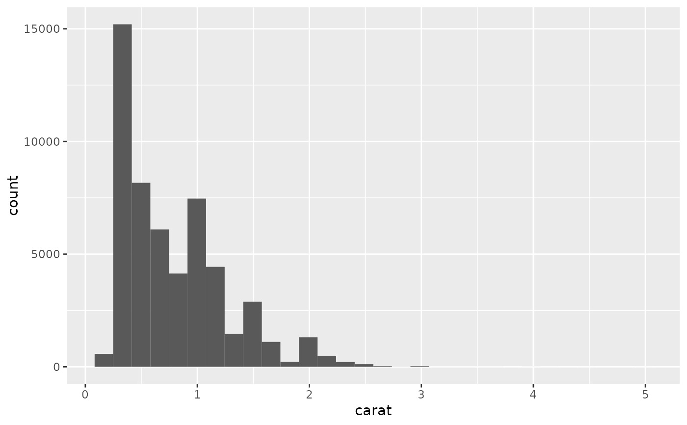
ggplot(diamonds, aes(carat)) +
geom_histogram()
#> `stat_bin()` using `bins = 30`. Pick better value with `binwidth`.
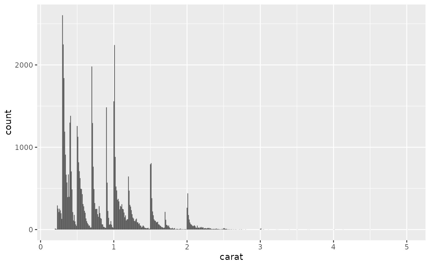
 ggplot(diamonds, aes(carat)) +
geom_histogram(binwidth = 0.01)
ggplot(diamonds, aes(carat)) +
geom_histogram(binwidth = 0.01)
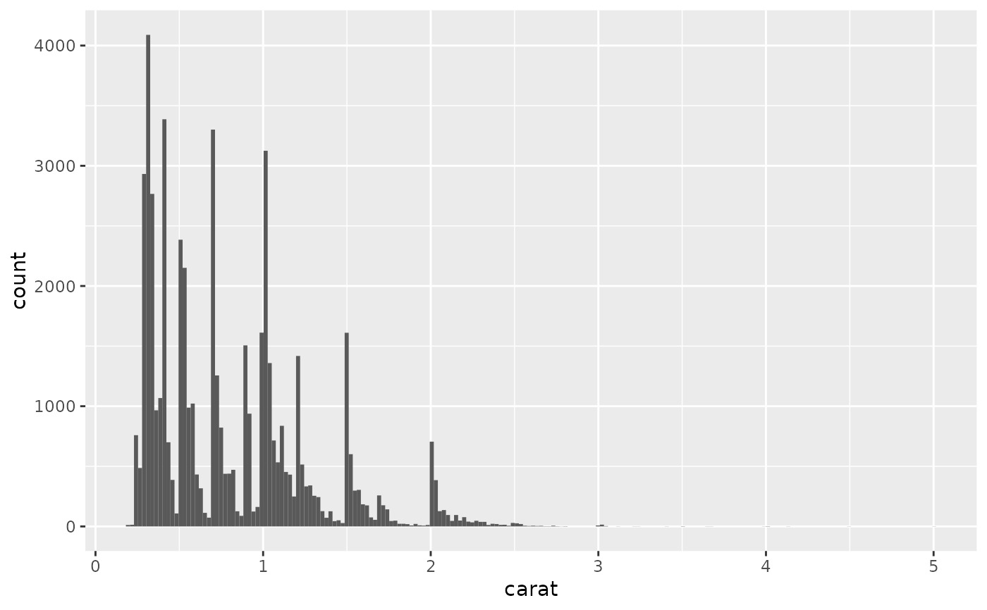
 ggplot(diamonds, aes(carat)) +
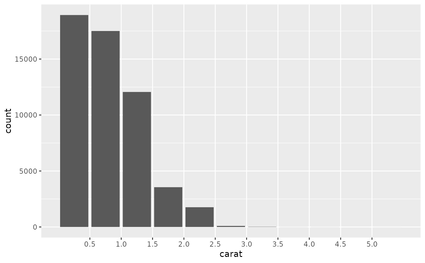
geom_histogram(bins = 200)
ggplot(diamonds, aes(carat)) +
geom_histogram(bins = 200)
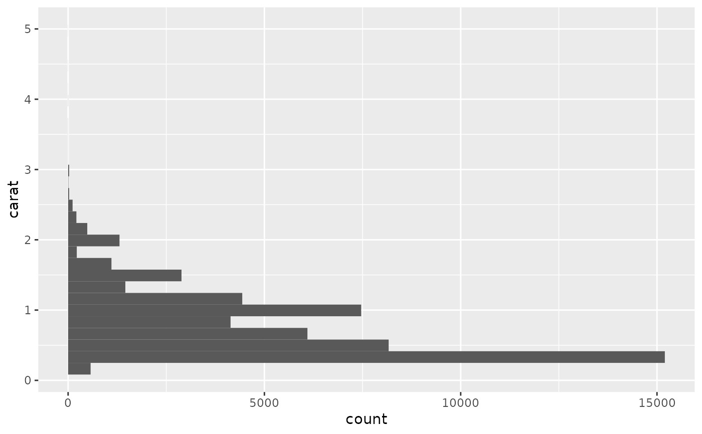
 # Map values to y to flip the orientation
ggplot(diamonds, aes(y = carat)) +
geom_histogram()
#> `stat_bin()` using `bins = 30`. Pick better value with `binwidth`.
# Map values to y to flip the orientation
ggplot(diamonds, aes(y = carat)) +
geom_histogram()
#> `stat_bin()` using `bins = 30`. Pick better value with `binwidth`.
 # For histograms with tick marks between each bin, use `geom_bar()` with
# `scale_x_binned()`.
ggplot(diamonds, aes(carat)) +
geom_bar() +
scale_x_binned()
# For histograms with tick marks between each bin, use `geom_bar()` with
# `scale_x_binned()`.
ggplot(diamonds, aes(carat)) +
geom_bar() +
scale_x_binned()
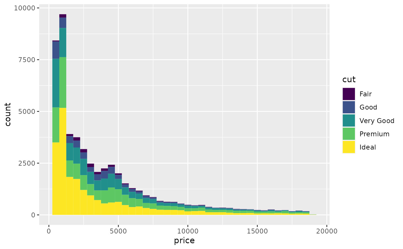
 # Rather than stacking histograms, it's easier to compare frequency
# polygons
ggplot(diamonds, aes(price, fill = cut)) +
geom_histogram(binwidth = 500)
# Rather than stacking histograms, it's easier to compare frequency
# polygons
ggplot(diamonds, aes(price, fill = cut)) +
geom_histogram(binwidth = 500)
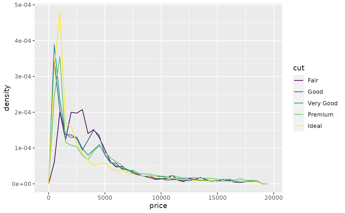
 ggplot(diamonds, aes(price, colour = cut)) +
geom_freqpoly(binwidth = 500)
ggplot(diamonds, aes(price, colour = cut)) +
geom_freqpoly(binwidth = 500)
 # To make it easier to compare distributions with very different counts,
# put density on the y axis instead of the default count
ggplot(diamonds, aes(price, after_stat(density), colour = cut)) +
geom_freqpoly(binwidth = 500)
# To make it easier to compare distributions with very different counts,
# put density on the y axis instead of the default count
ggplot(diamonds, aes(price, after_stat(density), colour = cut)) +
geom_freqpoly(binwidth = 500)
 if (require("ggplot2movies")) {
# Often we don't want the height of the bar to represent the
# count of observations, but the sum of some other variable.
# For example, the following plot shows the number of movies
# in each rating.
m <- ggplot(movies, aes(rating))
m + geom_histogram(binwidth = 0.1)
# If, however, we want to see the number of votes cast in each
# category, we need to weight by the votes variable
m +
geom_histogram(aes(weight = votes), binwidth = 0.1) +
ylab("votes")
# For transformed scales, binwidth applies to the transformed data.
# The bins have constant width on the transformed scale.
m +
geom_histogram() +
scale_x_log10()
m +
geom_histogram(binwidth = 0.05) +
scale_x_log10()
# For transformed coordinate systems, the binwidth applies to the
# raw data. The bins have constant width on the original scale.
# Using log scales does not work here, because the first
# bar is anchored at zero, and so when transformed becomes negative
# infinity. This is not a problem when transforming the scales, because
# no observations have 0 ratings.
m +
geom_histogram(boundary = 0) +
coord_trans(x = "log10")
# Use boundary = 0, to make sure we don't take sqrt of negative values
m +
geom_histogram(boundary = 0) +
coord_trans(x = "sqrt")
# You can also transform the y axis. Remember that the base of the bars
# has value 0, so log transformations are not appropriate
m <- ggplot(movies, aes(x = rating))
m +
geom_histogram(binwidth = 0.5) +
scale_y_sqrt()
}
if (require("ggplot2movies")) {
# Often we don't want the height of the bar to represent the
# count of observations, but the sum of some other variable.
# For example, the following plot shows the number of movies
# in each rating.
m <- ggplot(movies, aes(rating))
m + geom_histogram(binwidth = 0.1)
# If, however, we want to see the number of votes cast in each
# category, we need to weight by the votes variable
m +
geom_histogram(aes(weight = votes), binwidth = 0.1) +
ylab("votes")
# For transformed scales, binwidth applies to the transformed data.
# The bins have constant width on the transformed scale.
m +
geom_histogram() +
scale_x_log10()
m +
geom_histogram(binwidth = 0.05) +
scale_x_log10()
# For transformed coordinate systems, the binwidth applies to the
# raw data. The bins have constant width on the original scale.
# Using log scales does not work here, because the first
# bar is anchored at zero, and so when transformed becomes negative
# infinity. This is not a problem when transforming the scales, because
# no observations have 0 ratings.
m +
geom_histogram(boundary = 0) +
coord_trans(x = "log10")
# Use boundary = 0, to make sure we don't take sqrt of negative values
m +
geom_histogram(boundary = 0) +
coord_trans(x = "sqrt")
# You can also transform the y axis. Remember that the base of the bars
# has value 0, so log transformations are not appropriate
m <- ggplot(movies, aes(x = rating))
m +
geom_histogram(binwidth = 0.5) +
scale_y_sqrt()
}
 # You can specify a function for calculating binwidth, which is
# particularly useful when faceting along variables with
# different ranges because the function will be called once per facet
ggplot(economics_long, aes(value)) +
facet_wrap(~variable, scales = 'free_x') +
geom_histogram(binwidth = function(x) 2 * IQR(x) / (length(x)^(1/3)))
# You can specify a function for calculating binwidth, which is
# particularly useful when faceting along variables with
# different ranges because the function will be called once per facet
ggplot(economics_long, aes(value)) +
facet_wrap(~variable, scales = 'free_x') +
geom_histogram(binwidth = function(x) 2 * IQR(x) / (length(x)^(1/3)))

相关用法
- R ggplot2 geom_hex 二维箱计数的六边形热图
- R ggplot2 geom_qq 分位数-分位数图
- R ggplot2 geom_spoke 由位置、方向和距离参数化的线段
- R ggplot2 geom_quantile 分位数回归
- R ggplot2 geom_text 文本
- R ggplot2 geom_ribbon 函数区和面积图
- R ggplot2 geom_boxplot 盒须图(Tukey 风格)
- R ggplot2 geom_bar 条形图
- R ggplot2 geom_bin_2d 二维 bin 计数热图
- R ggplot2 geom_jitter 抖动点
- R ggplot2 geom_point 积分
- R ggplot2 geom_linerange 垂直间隔:线、横线和误差线
- R ggplot2 geom_blank 什么也不画
- R ggplot2 geom_path 连接观察结果
- R ggplot2 geom_violin 小提琴情节
- R ggplot2 geom_dotplot 点图
- R ggplot2 geom_errorbarh 水平误差线
- R ggplot2 geom_function 将函数绘制为连续曲线
- R ggplot2 geom_polygon 多边形
- R ggplot2 geom_tile 矩形
- R ggplot2 geom_segment 线段和曲线
- R ggplot2 geom_density_2d 二维密度估计的等值线
- R ggplot2 geom_map 参考Map中的多边形
- R ggplot2 geom_density 平滑密度估计
- R ggplot2 geom_abline 参考线:水平、垂直和对角线
注:本文由纯净天空筛选整理自Hadley Wickham等大神的英文原创作品 Histograms and frequency polygons。非经特殊声明,原始代码版权归原作者所有,本译文未经允许或授权,请勿转载或复制。