geom_rect() 和 geom_tile() 执行相同的操作,但参数化不同: geom_rect() 使用四个角的位置( xmin 、 xmax 、 ymin 和 ymax ),而 geom_tile() 使用图块的中心及其大小( x 、 y 、 width 、 height )。 geom_raster() 是所有图块大小相同时的高性能特殊情况。
用法
geom_raster(
  mapping = NULL,
  data = NULL,
  stat = "identity",
  position = "identity",
  ...,
  hjust = 0.5,
  vjust = 0.5,
  interpolate = FALSE,
  na.rm = FALSE,
  show.legend = NA,
  inherit.aes = TRUE
)

geom_rect(
  mapping = NULL,
  data = NULL,
  stat = "identity",
  position = "identity",
  ...,
  linejoin = "mitre",
  na.rm = FALSE,
  show.legend = NA,
  inherit.aes = TRUE
)

geom_tile(
  mapping = NULL,
  data = NULL,
  stat = "identity",
  position = "identity",
  ...,
  linejoin = "mitre",
  na.rm = FALSE,
  show.legend = NA,
  inherit.aes = TRUE
)
参数
- mapping
-
由
aes()创建的一组美学映射。如果指定且inherit.aes = TRUE(默认),它将与绘图顶层的默认映射组合。如果没有绘图映射,则必须提供mapping。 - data
-
该层要显示的数据。有以下三种选择:
如果默认为
NULL,则数据继承自ggplot()调用中指定的绘图数据。data.frame或其他对象将覆盖绘图数据。所有对象都将被强化以生成 DataFrame 。请参阅fortify()将为其创建变量。将使用单个参数(绘图数据)调用
function。返回值必须是data.frame,并将用作图层数据。可以从formula创建function(例如~ head(.x, 10))。 - stat
-
用于该层数据的统计变换,可以作为
ggprotoGeom子类,也可以作为命名去掉stat_前缀的统计数据的字符串(例如"count"而不是"stat_count") - position
-
位置调整,可以是命名调整的字符串(例如
"jitter"使用position_jitter),也可以是调用位置调整函数的结果。如果需要更改调整设置,请使用后者。 - ...
-
其他参数传递给
layer()。这些通常是美学,用于将美学设置为固定值,例如colour = "red"或size = 3。它们也可能是配对的 geom/stat 的参数。 - hjust, vjust
-
grob 的水平和垂直对齐。每个调整值应为 0 到 1 之间的数字。两者均默认为 0.5,使每个像素在其数据位置上居中。
- interpolate
-
如果
TRUE线性插值,如果FALSE(默认)不插值。 - na.rm
-
如果
FALSE,则默认缺失值将被删除并带有警告。如果TRUE,缺失值将被静默删除。 - show.legend
-
合乎逻辑的。该层是否应该包含在图例中?
NA(默认值)包括是否映射了任何美学。FALSE从不包含,而TRUE始终包含。它也可以是一个命名的逻辑向量,以精细地选择要显示的美学。 - inherit.aes
-
如果
FALSE,则覆盖默认美学,而不是与它们组合。这对于定义数据和美观的辅助函数最有用,并且不应继承默认绘图规范的行为,例如borders()。 - linejoin
-
线连接样式(圆形、斜接、斜角)。
美学
geom_tile() 理解以下美学(所需的美学以粗体显示):
-
x -
y -
alpha -
colour -
fill -
group -
height -
linetype -
linewidth -
width
请注意, geom_raster() 忽略 colour 。
在 vignette("ggplot2-specs") 中了解有关设置这些美学的更多信息。
例子
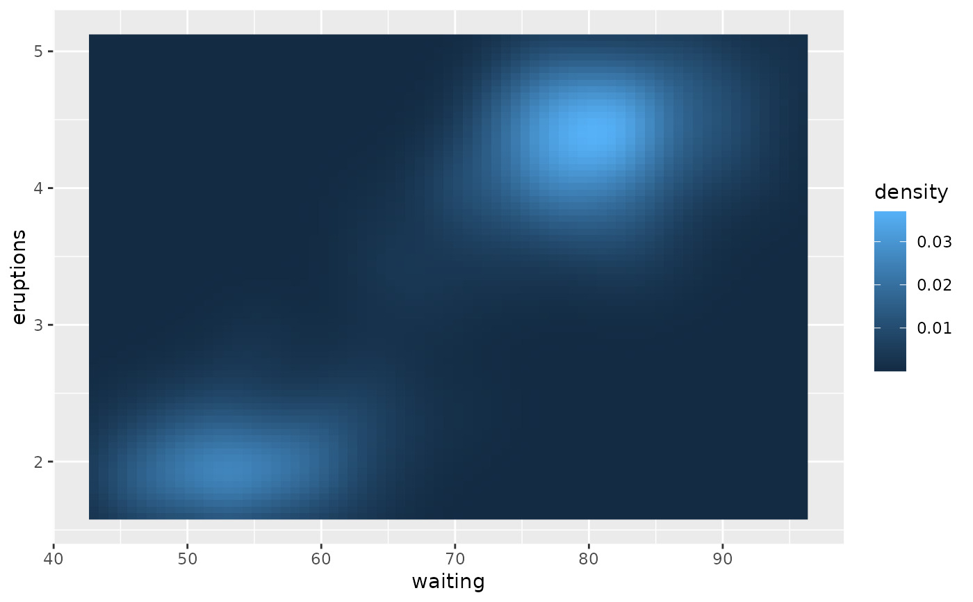
# The most common use for rectangles is to draw a surface. You always want
# to use geom_raster here because it's so much faster, and produces
# smaller output when saving to PDF
ggplot(faithfuld, aes(waiting, eruptions)) +
geom_raster(aes(fill = density))
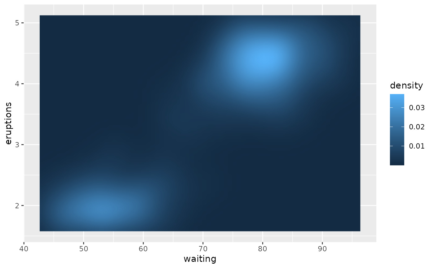
 # Interpolation smooths the surface & is most helpful when rendering images.
ggplot(faithfuld, aes(waiting, eruptions)) +
geom_raster(aes(fill = density), interpolate = TRUE)
# Interpolation smooths the surface & is most helpful when rendering images.
ggplot(faithfuld, aes(waiting, eruptions)) +
geom_raster(aes(fill = density), interpolate = TRUE)
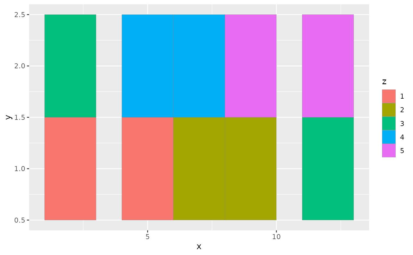
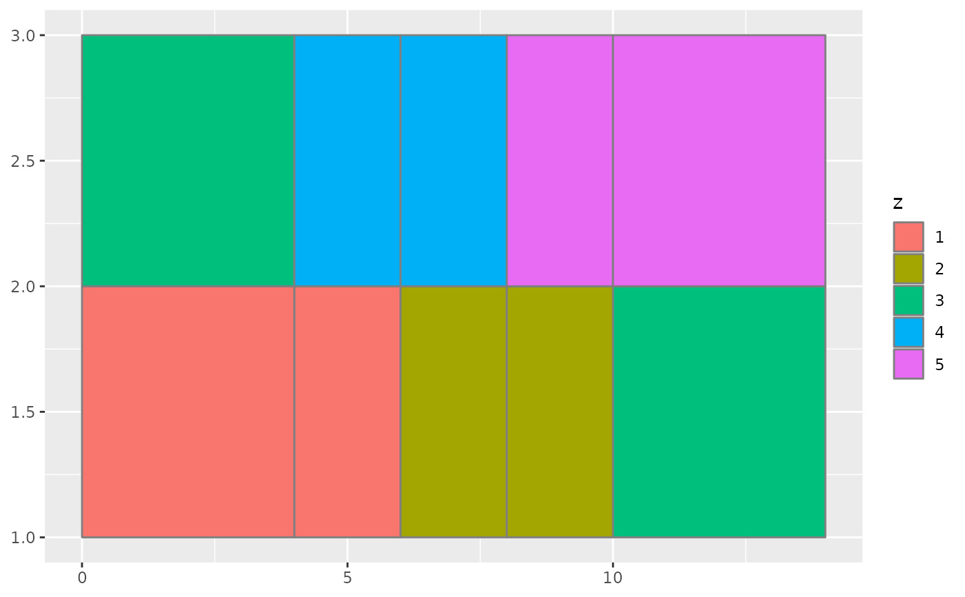
 # If you want to draw arbitrary rectangles, use geom_tile() or geom_rect()
df <- data.frame(
x = rep(c(2, 5, 7, 9, 12), 2),
y = rep(c(1, 2), each = 5),
z = factor(rep(1:5, each = 2)),
w = rep(diff(c(0, 4, 6, 8, 10, 14)), 2)
)
ggplot(df, aes(x, y)) +
geom_tile(aes(fill = z), colour = "grey50")
# If you want to draw arbitrary rectangles, use geom_tile() or geom_rect()
df <- data.frame(
x = rep(c(2, 5, 7, 9, 12), 2),
y = rep(c(1, 2), each = 5),
z = factor(rep(1:5, each = 2)),
w = rep(diff(c(0, 4, 6, 8, 10, 14)), 2)
)
ggplot(df, aes(x, y)) +
geom_tile(aes(fill = z), colour = "grey50")
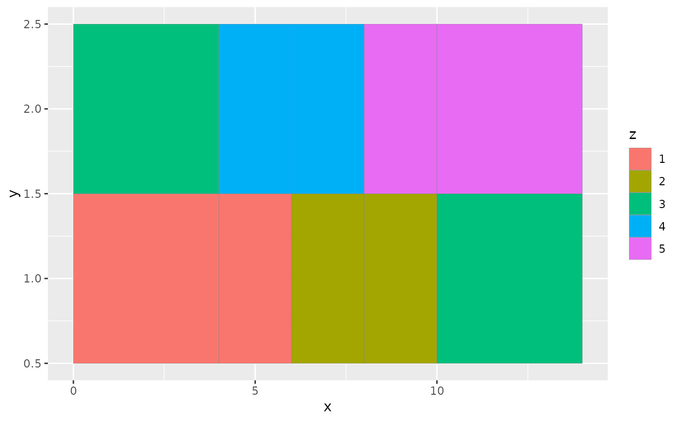
 ggplot(df, aes(x, y, width = w)) +
geom_tile(aes(fill = z), colour = "grey50")
ggplot(df, aes(x, y, width = w)) +
geom_tile(aes(fill = z), colour = "grey50")
 ggplot(df, aes(xmin = x - w / 2, xmax = x + w / 2, ymin = y, ymax = y + 1)) +
geom_rect(aes(fill = z), colour = "grey50")
ggplot(df, aes(xmin = x - w / 2, xmax = x + w / 2, ymin = y, ymax = y + 1)) +
geom_rect(aes(fill = z), colour = "grey50")
 # \donttest{
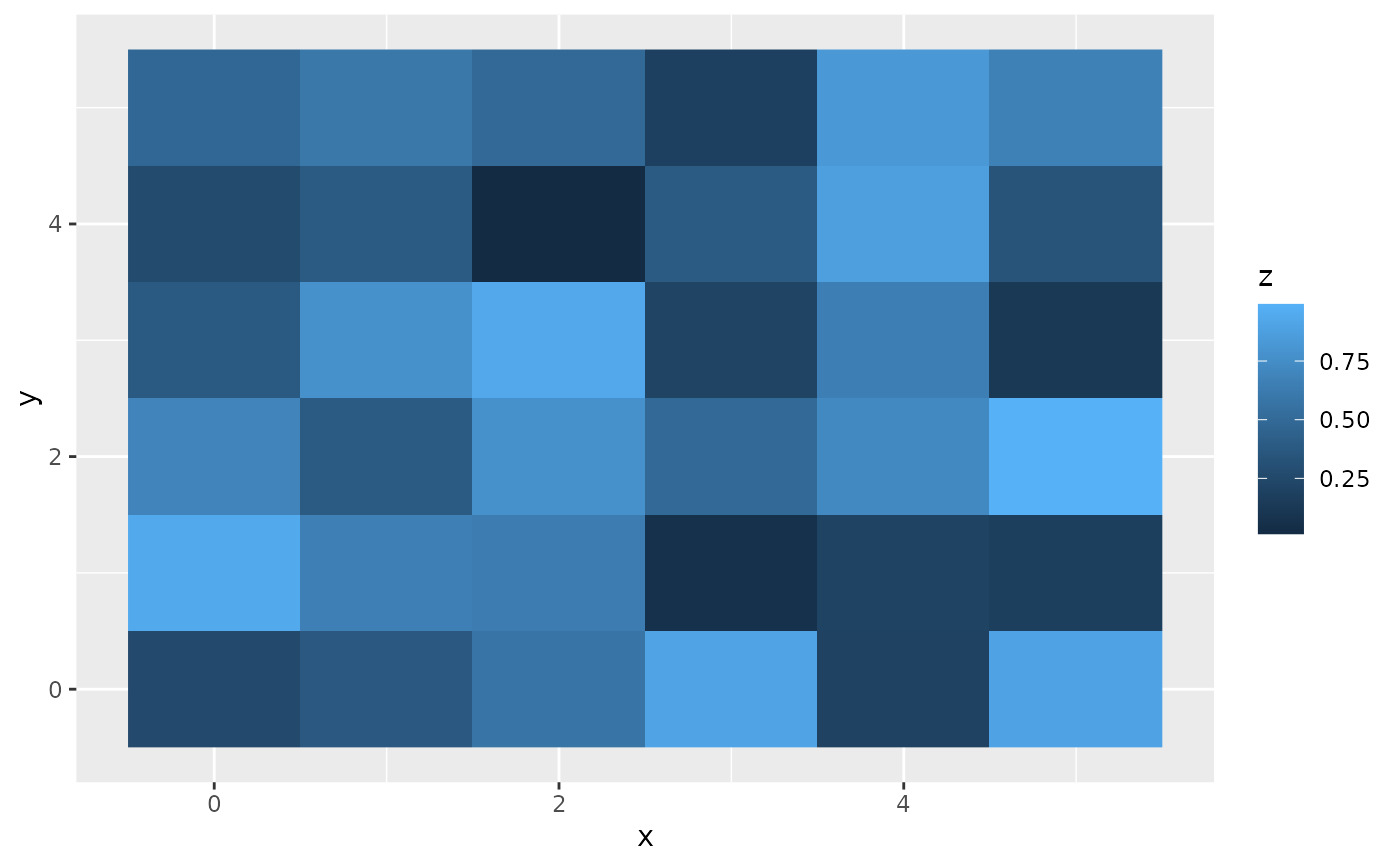
# Justification controls where the cells are anchored
df <- expand.grid(x = 0:5, y = 0:5)
set.seed(1)
df$z <- runif(nrow(df))
# default is compatible with geom_tile()
ggplot(df, aes(x, y, fill = z)) +
geom_raster()
# \donttest{
# Justification controls where the cells are anchored
df <- expand.grid(x = 0:5, y = 0:5)
set.seed(1)
df$z <- runif(nrow(df))
# default is compatible with geom_tile()
ggplot(df, aes(x, y, fill = z)) +
geom_raster()
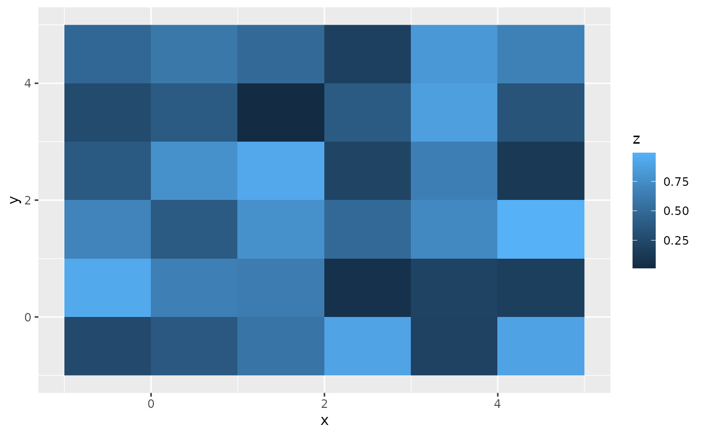
 # zero padding
ggplot(df, aes(x, y, fill = z)) +
geom_raster(hjust = 0, vjust = 0)
# zero padding
ggplot(df, aes(x, y, fill = z)) +
geom_raster(hjust = 0, vjust = 0)
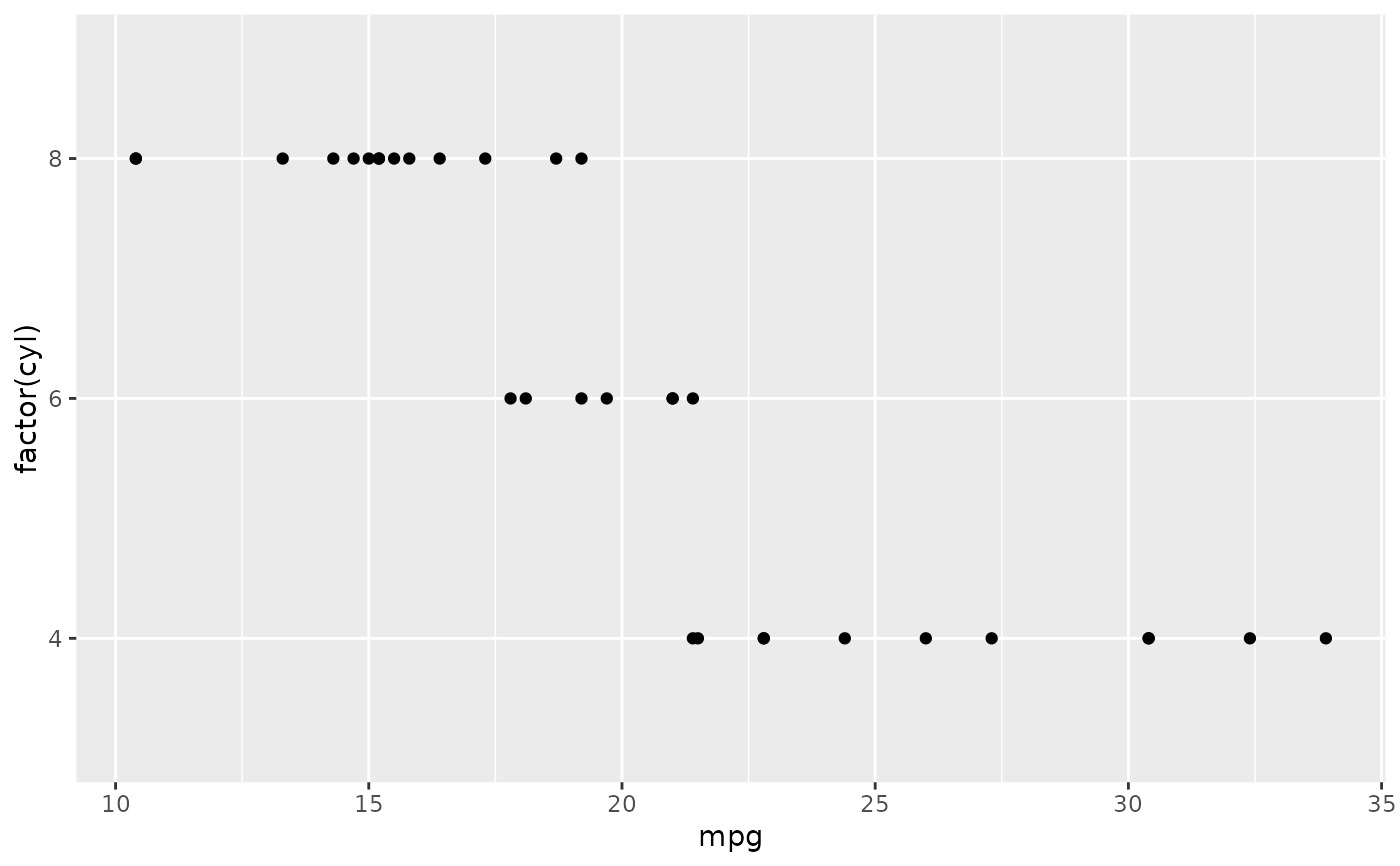
 # Inspired by the image-density plots of Ken Knoblauch
cars <- ggplot(mtcars, aes(mpg, factor(cyl)))
cars + geom_point()
# Inspired by the image-density plots of Ken Knoblauch
cars <- ggplot(mtcars, aes(mpg, factor(cyl)))
cars + geom_point()
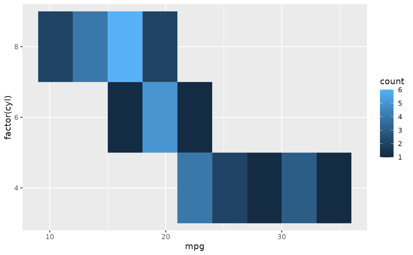
 cars + stat_bin2d(aes(fill = after_stat(count)), binwidth = c(3,1))
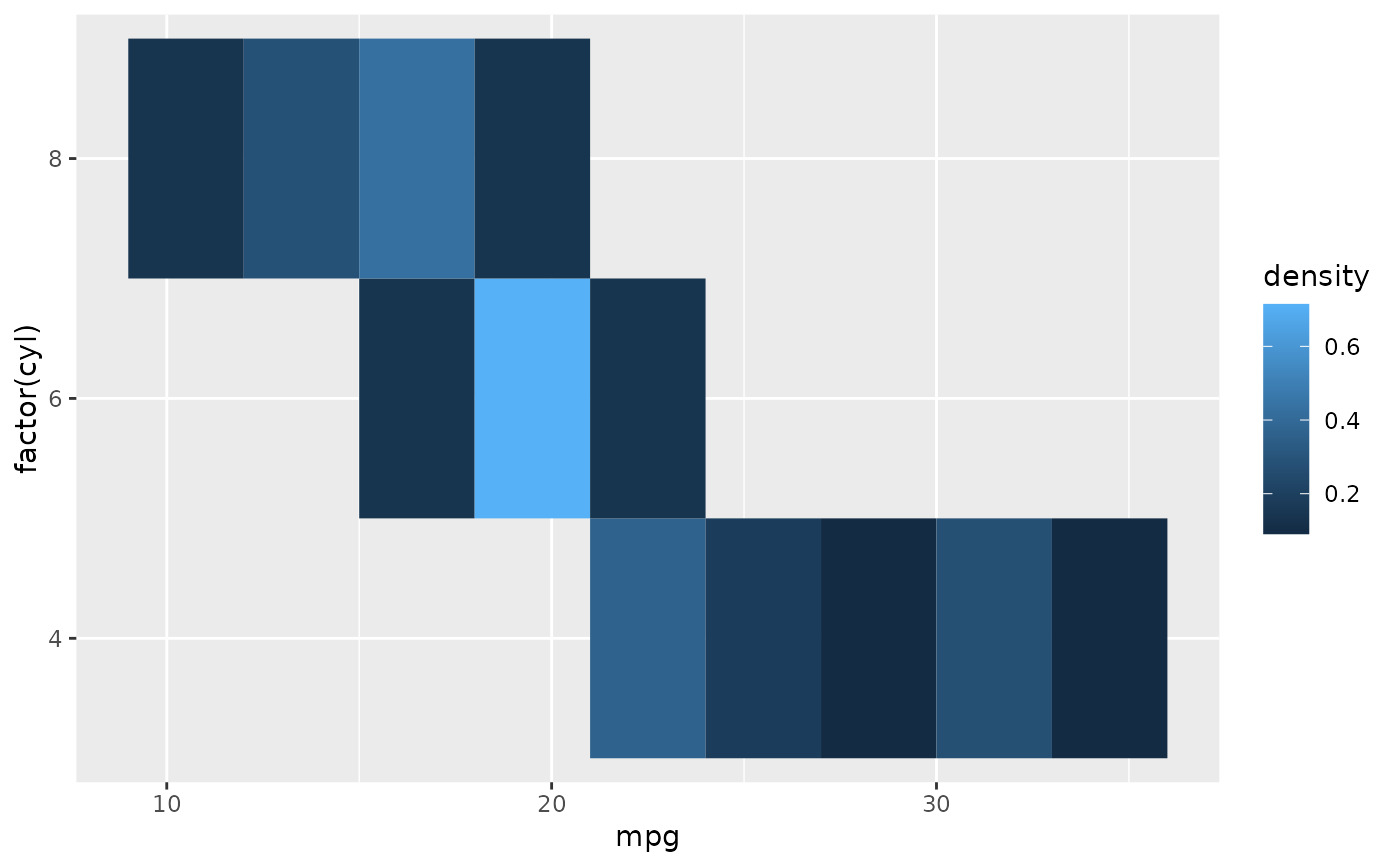
 cars + stat_bin2d(aes(fill = after_stat(density)), binwidth = c(3,1))
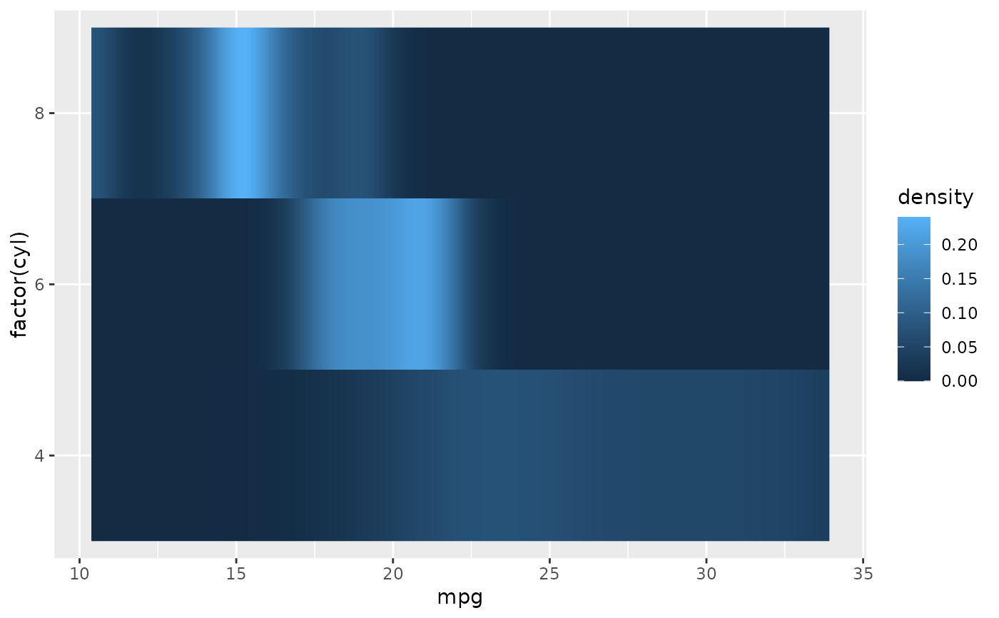
 cars +
stat_density(
aes(fill = after_stat(density)),
geom = "raster",
position = "identity"
)
cars +
stat_density(
aes(fill = after_stat(density)),
geom = "raster",
position = "identity"
)
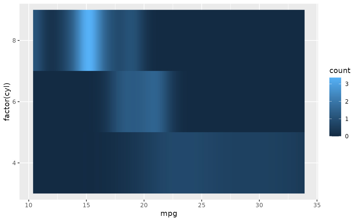
 cars +
stat_density(
aes(fill = after_stat(count)),
geom = "raster",
position = "identity"
)
cars +
stat_density(
aes(fill = after_stat(count)),
geom = "raster",
position = "identity"
)
 # }
# }
相关用法
- R ggplot2 geom_text 文本
- R ggplot2 geom_qq 分位数-分位数图
- R ggplot2 geom_spoke 由位置、方向和距离参数化的线段
- R ggplot2 geom_quantile 分位数回归
- R ggplot2 geom_ribbon 函数区和面积图
- R ggplot2 geom_boxplot 盒须图(Tukey 风格)
- R ggplot2 geom_hex 二维箱计数的六边形热图
- R ggplot2 geom_bar 条形图
- R ggplot2 geom_bin_2d 二维 bin 计数热图
- R ggplot2 geom_jitter 抖动点
- R ggplot2 geom_point 积分
- R ggplot2 geom_linerange 垂直间隔:线、横线和误差线
- R ggplot2 geom_blank 什么也不画
- R ggplot2 geom_path 连接观察结果
- R ggplot2 geom_violin 小提琴情节
- R ggplot2 geom_dotplot 点图
- R ggplot2 geom_errorbarh 水平误差线
- R ggplot2 geom_function 将函数绘制为连续曲线
- R ggplot2 geom_polygon 多边形
- R ggplot2 geom_histogram 直方图和频数多边形
- R ggplot2 geom_segment 线段和曲线
- R ggplot2 geom_density_2d 二维密度估计的等值线
- R ggplot2 geom_map 参考Map中的多边形
- R ggplot2 geom_density 平滑密度估计
- R ggplot2 geom_abline 参考线:水平、垂直和对角线
注:本文由纯净天空筛选整理自Hadley Wickham等大神的英文原创作品 Rectangles。非经特殊声明,原始代码版权归原作者所有,本译文未经允许或授权,请勿转载或复制。