在点图中,点的宽度对应于分箱宽度(或最大宽度,取决于分箱算法),并且点堆叠在一起,每个点代表一个观察值。
用法
geom_dotplot(
  mapping = NULL,
  data = NULL,
  position = "identity",
  ...,
  binwidth = NULL,
  binaxis = "x",
  method = "dotdensity",
  binpositions = "bygroup",
  stackdir = "up",
  stackratio = 1,
  dotsize = 1,
  stackgroups = FALSE,
  origin = NULL,
  right = TRUE,
  width = 0.9,
  drop = FALSE,
  na.rm = FALSE,
  show.legend = NA,
  inherit.aes = TRUE
)
参数
- mapping
-
由
aes()创建的一组美学映射。如果指定且inherit.aes = TRUE(默认),它将与绘图顶层的默认映射组合。如果没有绘图映射,则必须提供mapping。 - data
-
该层要显示的数据。有以下三种选择:
如果默认为
NULL,则数据继承自ggplot()调用中指定的绘图数据。data.frame或其他对象将覆盖绘图数据。所有对象都将被强化以生成 DataFrame 。请参阅fortify()将为其创建变量。将使用单个参数(绘图数据)调用
function。返回值必须是data.frame,并将用作图层数据。可以从formula创建function(例如~ head(.x, 10))。 - position
-
位置调整,可以是命名调整的字符串(例如
"jitter"使用position_jitter),也可以是调用位置调整函数的结果。如果需要更改调整设置,请使用后者。 - ...
-
其他参数传递给
layer()。这些通常是美学,用于将美学设置为固定值,例如colour = "red"或size = 3。它们也可能是配对的 geom/stat 的参数。 - binwidth
-
当
method为"dotdensity" 时,指定最大bin 宽度。当method为"histodot" 时,指定bin 宽度。默认为数据范围的 1/30 - binaxis
-
分箱沿的轴,"x"(默认)或"y"
- method
-
"dotdensity"(默认)用于 dot-density 分箱,或 "histodot" 用于固定分箱宽度(如 stat_bin)
- binpositions
-
当
method为"dotdensity" 时,"bygroup"(默认)分别确定每个组的bin 位置。 "all" 确定所有数据放在一起后的 bin 的位置;这用于跨多个组对齐点堆栈。 - stackdir
-
向哪个方向堆叠点。 "up"(默认)、"down"、"center"、"centerwhole"(居中,但点对齐)
- stackratio
-
点堆叠的距离有多近。默认值为 1,即点刚好接触。对于更近、重叠的点,请使用较小的值。
- dotsize
-
相对于
binwidth的点的直径,默认1。 - stackgroups
-
点应该跨组堆叠吗?这具有
position = "stack"应该具有的效果,但不能(因为该几何对象具有一些奇怪的属性)。 - origin
-
当
method为"histodot"时,第一个bin的原点 - right
-
当
method为"histodot"时,区间应该在右边闭合(a,b],还是不闭合[a,b) - width
-
当
binaxis为"y"时,用于躲避的点堆叠的间距。 - drop
-
如果为 TRUE,则删除所有计数为零的箱子
- na.rm
-
如果
FALSE,则默认缺失值将被删除并带有警告。如果TRUE,缺失值将被静默删除。 - show.legend
-
合乎逻辑的。该层是否应该包含在图例中?
NA(默认值)包括是否映射了任何美学。FALSE从不包含,而TRUE始终包含。它也可以是一个命名的逻辑向量,以精细地选择要显示的美学。 - inherit.aes
-
如果
FALSE,则覆盖默认美学,而不是与它们组合。这对于定义数据和美观的辅助函数最有用,并且不应继承默认绘图规范的行为,例如borders()。
细节
有两种基本方法:dot-density 和 histodot。对于 dot-density 分箱,分箱位置由数据和 binwidth 确定,binwidth 是每个分箱的最大宽度。有关 dot-density 分箱算法的详细信息,请参阅 Wilkinson (1999)。通过 histodot binning,箱具有固定的位置和固定的宽度,很像直方图。
当沿 x 轴分箱并沿 y 轴堆叠时,由于 ggplot2 的技术限制,y 轴上的数字没有意义。您可以隐藏 y 轴(如示例之一所示),或手动缩放它以匹配点数。
美学
geom_dotplot() 理解以下美学(所需的美学以粗体显示):
-
x -
y -
alpha -
colour -
fill -
group -
linetype -
stroke
在 vignette("ggplot2-specs") 中了解有关设置这些美学的更多信息。
计算变量
这些是由层的 'stat' 部分计算的,可以使用 delayed evaluation 访问。
-
after_stat(x)
每个 bin 的中心,如果binaxis是"x". -
after_stat(y)
每个 bin 的中心,如果binaxis是"x". -
after_stat(binwidth)
如果方法是每个 bin 的最大宽度"dotdensity";如果方法是每个 bin 的宽度"histodot". -
after_stat(count)
bin 中的点数。 -
after_stat(ncount)
计数,缩放至最大值 1。 -
after_stat(density)
bin 中点的密度,缩放至积分为 1,如果方法是"histodot". -
after_stat(ndensity)
密度,缩放到最大值 1,如果方法是"histodot".
例子
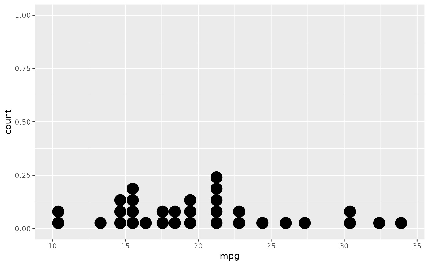
ggplot(mtcars, aes(x = mpg)) +
geom_dotplot()
#> Bin width defaults to 1/30 of the range of the data. Pick better value
#> with `binwidth`.
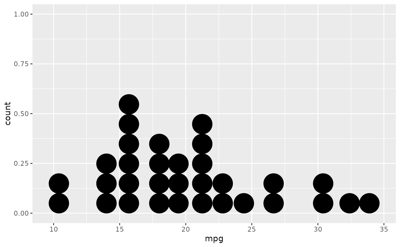
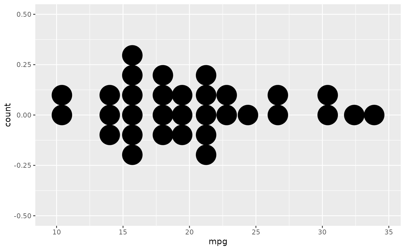
 ggplot(mtcars, aes(x = mpg)) +
geom_dotplot(binwidth = 1.5)
ggplot(mtcars, aes(x = mpg)) +
geom_dotplot(binwidth = 1.5)
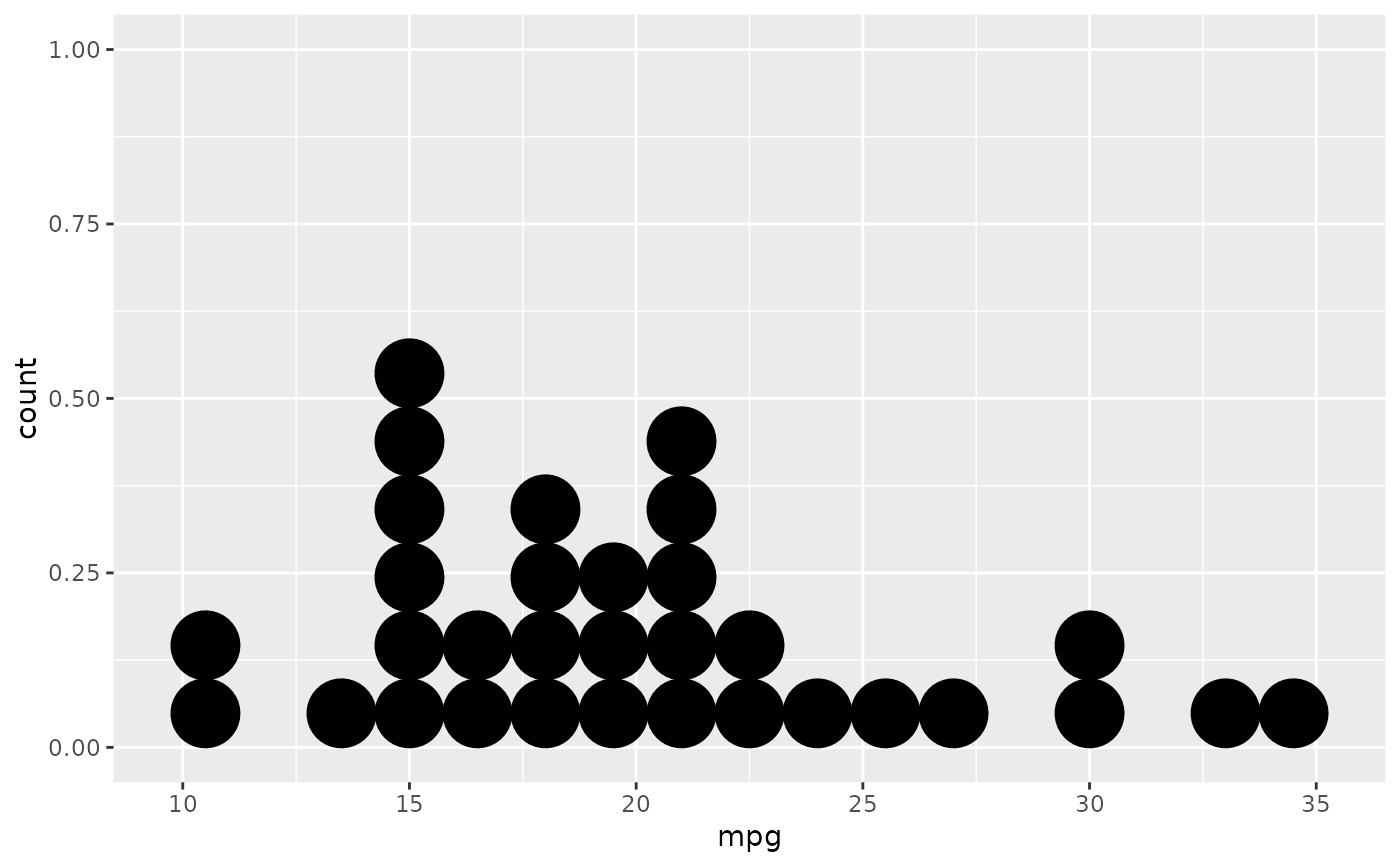
 # Use fixed-width bins
ggplot(mtcars, aes(x = mpg)) +
geom_dotplot(method="histodot", binwidth = 1.5)
# Use fixed-width bins
ggplot(mtcars, aes(x = mpg)) +
geom_dotplot(method="histodot", binwidth = 1.5)
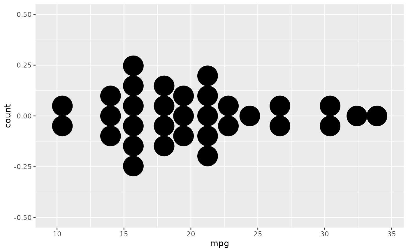
 # Some other stacking methods
ggplot(mtcars, aes(x = mpg)) +
geom_dotplot(binwidth = 1.5, stackdir = "center")
# Some other stacking methods
ggplot(mtcars, aes(x = mpg)) +
geom_dotplot(binwidth = 1.5, stackdir = "center")
 ggplot(mtcars, aes(x = mpg)) +
geom_dotplot(binwidth = 1.5, stackdir = "centerwhole")
ggplot(mtcars, aes(x = mpg)) +
geom_dotplot(binwidth = 1.5, stackdir = "centerwhole")
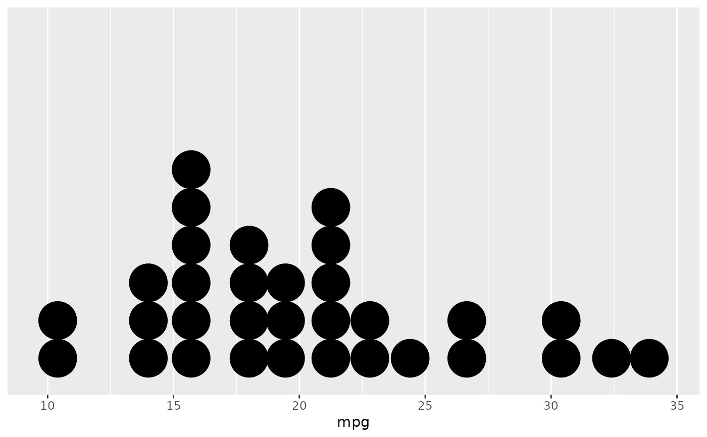
 # y axis isn't really meaningful, so hide it
ggplot(mtcars, aes(x = mpg)) + geom_dotplot(binwidth = 1.5) +
scale_y_continuous(NULL, breaks = NULL)
# y axis isn't really meaningful, so hide it
ggplot(mtcars, aes(x = mpg)) + geom_dotplot(binwidth = 1.5) +
scale_y_continuous(NULL, breaks = NULL)
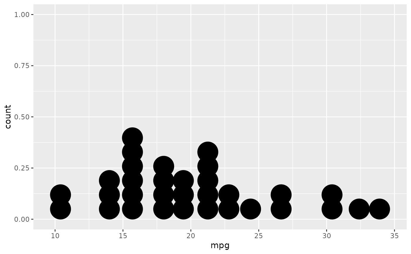
 # Overlap dots vertically
ggplot(mtcars, aes(x = mpg)) +
geom_dotplot(binwidth = 1.5, stackratio = .7)
# Overlap dots vertically
ggplot(mtcars, aes(x = mpg)) +
geom_dotplot(binwidth = 1.5, stackratio = .7)
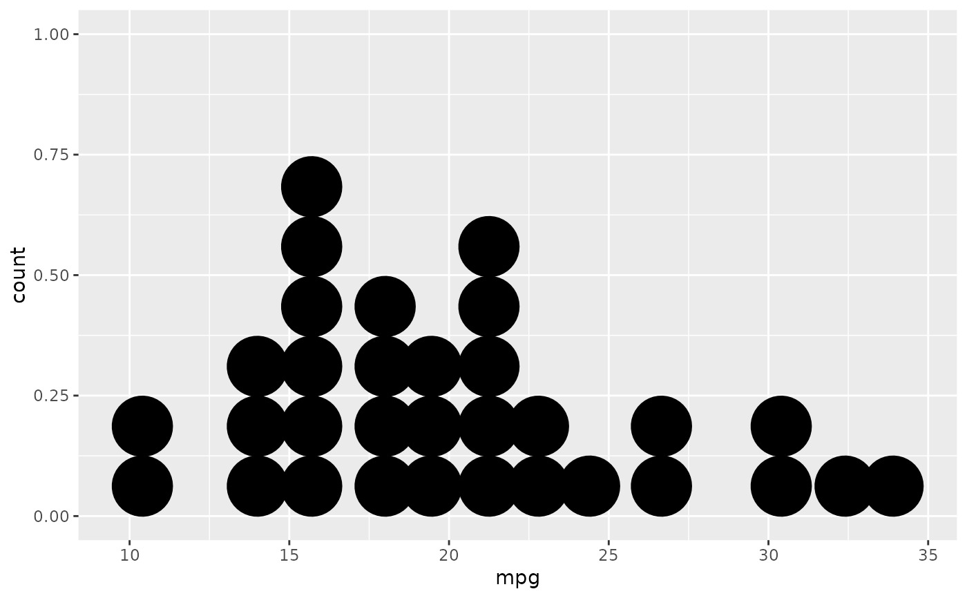
 # Expand dot diameter
ggplot(mtcars, aes(x = mpg)) +
geom_dotplot(binwidth = 1.5, dotsize = 1.25)
# Expand dot diameter
ggplot(mtcars, aes(x = mpg)) +
geom_dotplot(binwidth = 1.5, dotsize = 1.25)
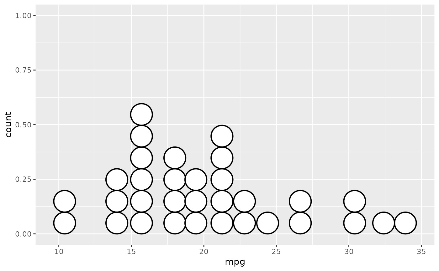
 # Change dot fill colour, stroke width
ggplot(mtcars, aes(x = mpg)) +
geom_dotplot(binwidth = 1.5, fill = "white", stroke = 2)
# Change dot fill colour, stroke width
ggplot(mtcars, aes(x = mpg)) +
geom_dotplot(binwidth = 1.5, fill = "white", stroke = 2)
 # \donttest{
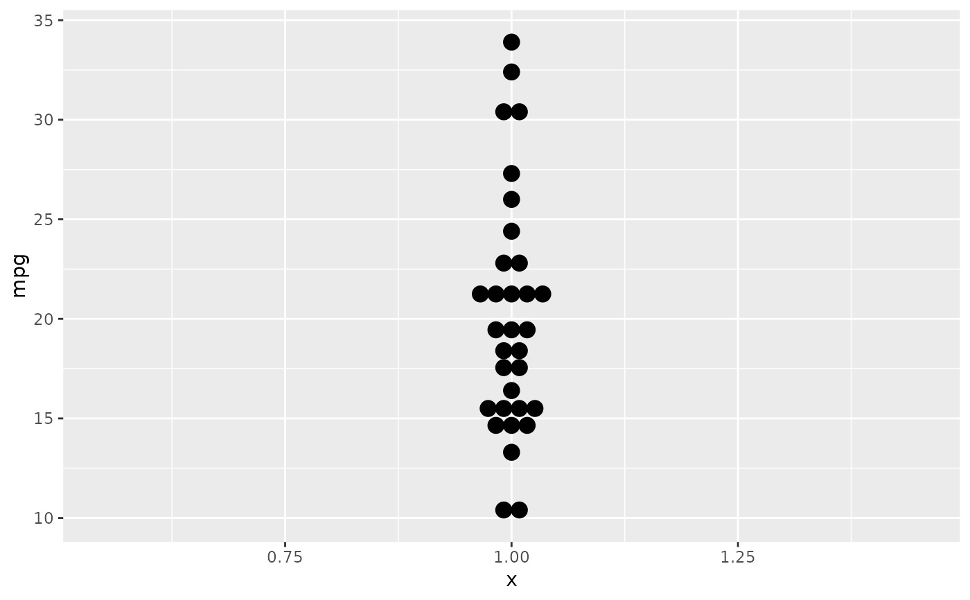
# Examples with stacking along y axis instead of x
ggplot(mtcars, aes(x = 1, y = mpg)) +
geom_dotplot(binaxis = "y", stackdir = "center")
#> Bin width defaults to 1/30 of the range of the data. Pick better value
#> with `binwidth`.
# \donttest{
# Examples with stacking along y axis instead of x
ggplot(mtcars, aes(x = 1, y = mpg)) +
geom_dotplot(binaxis = "y", stackdir = "center")
#> Bin width defaults to 1/30 of the range of the data. Pick better value
#> with `binwidth`.
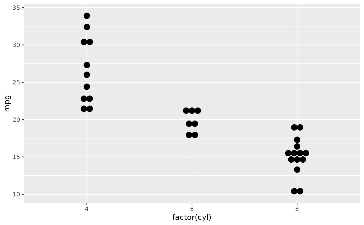
 ggplot(mtcars, aes(x = factor(cyl), y = mpg)) +
geom_dotplot(binaxis = "y", stackdir = "center")
#> Bin width defaults to 1/30 of the range of the data. Pick better value
#> with `binwidth`.
ggplot(mtcars, aes(x = factor(cyl), y = mpg)) +
geom_dotplot(binaxis = "y", stackdir = "center")
#> Bin width defaults to 1/30 of the range of the data. Pick better value
#> with `binwidth`.
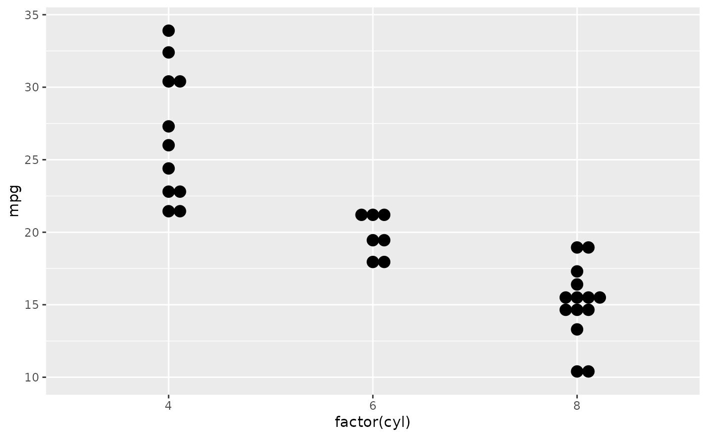
 ggplot(mtcars, aes(x = factor(cyl), y = mpg)) +
geom_dotplot(binaxis = "y", stackdir = "centerwhole")
#> Bin width defaults to 1/30 of the range of the data. Pick better value
#> with `binwidth`.
ggplot(mtcars, aes(x = factor(cyl), y = mpg)) +
geom_dotplot(binaxis = "y", stackdir = "centerwhole")
#> Bin width defaults to 1/30 of the range of the data. Pick better value
#> with `binwidth`.
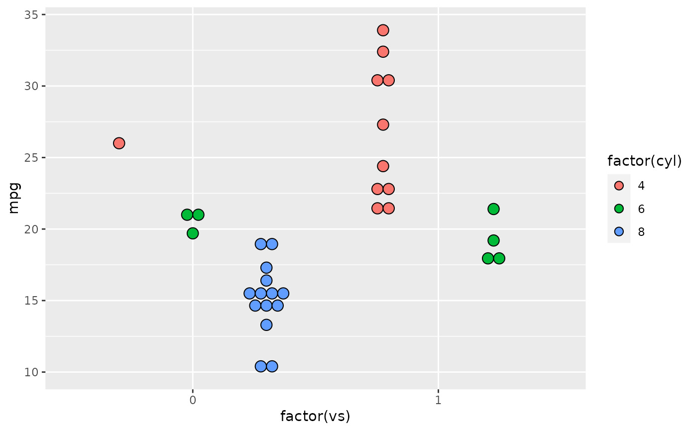
 ggplot(mtcars, aes(x = factor(vs), fill = factor(cyl), y = mpg)) +
geom_dotplot(binaxis = "y", stackdir = "center", position = "dodge")
#> Bin width defaults to 1/30 of the range of the data. Pick better value
#> with `binwidth`.
ggplot(mtcars, aes(x = factor(vs), fill = factor(cyl), y = mpg)) +
geom_dotplot(binaxis = "y", stackdir = "center", position = "dodge")
#> Bin width defaults to 1/30 of the range of the data. Pick better value
#> with `binwidth`.
 # binpositions="all" ensures that the bins are aligned between groups
ggplot(mtcars, aes(x = factor(am), y = mpg)) +
geom_dotplot(binaxis = "y", stackdir = "center", binpositions="all")
#> Bin width defaults to 1/30 of the range of the data. Pick better value
#> with `binwidth`.
# binpositions="all" ensures that the bins are aligned between groups
ggplot(mtcars, aes(x = factor(am), y = mpg)) +
geom_dotplot(binaxis = "y", stackdir = "center", binpositions="all")
#> Bin width defaults to 1/30 of the range of the data. Pick better value
#> with `binwidth`.
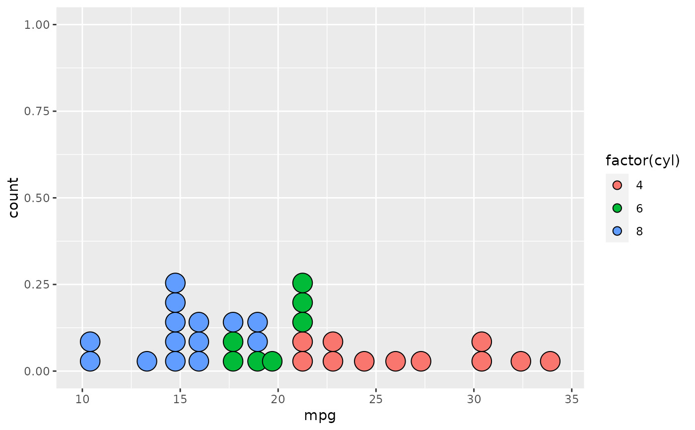
 # Stacking multiple groups, with different fill
ggplot(mtcars, aes(x = mpg, fill = factor(cyl))) +
geom_dotplot(stackgroups = TRUE, binwidth = 1, binpositions = "all")
# Stacking multiple groups, with different fill
ggplot(mtcars, aes(x = mpg, fill = factor(cyl))) +
geom_dotplot(stackgroups = TRUE, binwidth = 1, binpositions = "all")
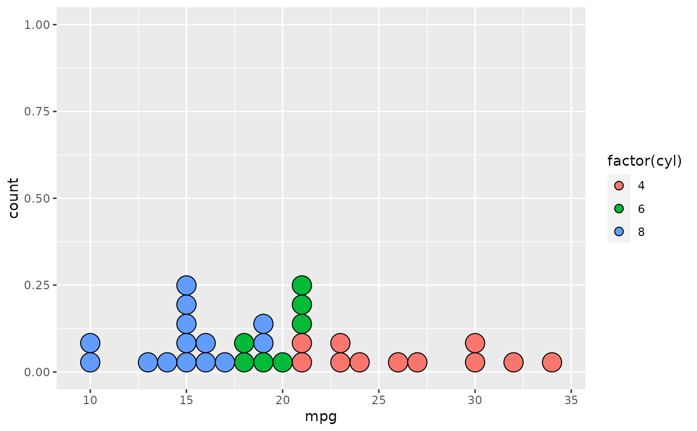
 ggplot(mtcars, aes(x = mpg, fill = factor(cyl))) +
geom_dotplot(stackgroups = TRUE, binwidth = 1, method = "histodot")
ggplot(mtcars, aes(x = mpg, fill = factor(cyl))) +
geom_dotplot(stackgroups = TRUE, binwidth = 1, method = "histodot")
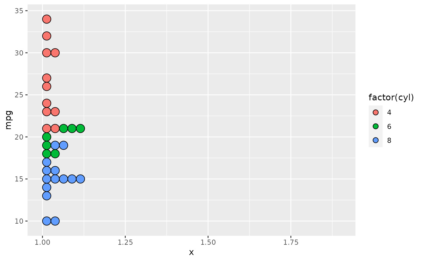
 ggplot(mtcars, aes(x = 1, y = mpg, fill = factor(cyl))) +
geom_dotplot(binaxis = "y", stackgroups = TRUE, binwidth = 1, method = "histodot")
ggplot(mtcars, aes(x = 1, y = mpg, fill = factor(cyl))) +
geom_dotplot(binaxis = "y", stackgroups = TRUE, binwidth = 1, method = "histodot")
 # }
# }
相关用法
- R ggplot2 geom_density_2d 二维密度估计的等值线
- R ggplot2 geom_density 平滑密度估计
- R ggplot2 geom_qq 分位数-分位数图
- R ggplot2 geom_spoke 由位置、方向和距离参数化的线段
- R ggplot2 geom_quantile 分位数回归
- R ggplot2 geom_text 文本
- R ggplot2 geom_ribbon 函数区和面积图
- R ggplot2 geom_boxplot 盒须图(Tukey 风格)
- R ggplot2 geom_hex 二维箱计数的六边形热图
- R ggplot2 geom_bar 条形图
- R ggplot2 geom_bin_2d 二维 bin 计数热图
- R ggplot2 geom_jitter 抖动点
- R ggplot2 geom_point 积分
- R ggplot2 geom_linerange 垂直间隔:线、横线和误差线
- R ggplot2 geom_blank 什么也不画
- R ggplot2 geom_path 连接观察结果
- R ggplot2 geom_violin 小提琴情节
- R ggplot2 geom_errorbarh 水平误差线
- R ggplot2 geom_function 将函数绘制为连续曲线
- R ggplot2 geom_polygon 多边形
- R ggplot2 geom_histogram 直方图和频数多边形
- R ggplot2 geom_tile 矩形
- R ggplot2 geom_segment 线段和曲线
- R ggplot2 geom_map 参考Map中的多边形
- R ggplot2 geom_abline 参考线:水平、垂直和对角线
注:本文由纯净天空筛选整理自Hadley Wickham等大神的英文原创作品 Dot plot。非经特殊声明,原始代码版权归原作者所有,本译文未经允许或授权,请勿转载或复制。