在點圖中,點的寬度對應於分箱寬度(或最大寬度,取決於分箱算法),並且點堆疊在一起,每個點代表一個觀察值。
用法
geom_dotplot(
  mapping = NULL,
  data = NULL,
  position = "identity",
  ...,
  binwidth = NULL,
  binaxis = "x",
  method = "dotdensity",
  binpositions = "bygroup",
  stackdir = "up",
  stackratio = 1,
  dotsize = 1,
  stackgroups = FALSE,
  origin = NULL,
  right = TRUE,
  width = 0.9,
  drop = FALSE,
  na.rm = FALSE,
  show.legend = NA,
  inherit.aes = TRUE
)
參數
- mapping
-
由
aes()創建的一組美學映射。如果指定且inherit.aes = TRUE(默認),它將與繪圖頂層的默認映射組合。如果沒有繪圖映射,則必須提供mapping。 - data
-
該層要顯示的數據。有以下三種選擇:
如果默認為
NULL,則數據繼承自ggplot()調用中指定的繪圖數據。data.frame或其他對象將覆蓋繪圖數據。所有對象都將被強化以生成 DataFrame 。請參閱fortify()將為其創建變量。將使用單個參數(繪圖數據)調用
function。返回值必須是data.frame,並將用作圖層數據。可以從formula創建function(例如~ head(.x, 10))。 - position
-
位置調整,可以是命名調整的字符串(例如
"jitter"使用position_jitter),也可以是調用位置調整函數的結果。如果需要更改調整設置,請使用後者。 - ...
-
其他參數傳遞給
layer()。這些通常是美學,用於將美學設置為固定值,例如colour = "red"或size = 3。它們也可能是配對的 geom/stat 的參數。 - binwidth
-
當
method為"dotdensity" 時,指定最大bin 寬度。當method為"histodot" 時,指定bin 寬度。默認為數據範圍的 1/30 - binaxis
-
分箱沿的軸,"x"(默認)或"y"
- method
-
"dotdensity"(默認)用於 dot-density 分箱,或 "histodot" 用於固定分箱寬度(如 stat_bin)
- binpositions
-
當
method為"dotdensity" 時,"bygroup"(默認)分別確定每個組的bin 位置。 "all" 確定所有數據放在一起後的 bin 的位置;這用於跨多個組對齊點堆棧。 - stackdir
-
向哪個方向堆疊點。 "up"(默認)、"down"、"center"、"centerwhole"(居中,但點對齊)
- stackratio
-
點堆疊的距離有多近。默認值為 1,即點剛好接觸。對於更近、重疊的點,請使用較小的值。
- dotsize
-
相對於
binwidth的點的直徑,默認1。 - stackgroups
-
點應該跨組堆疊嗎?這具有
position = "stack"應該具有的效果,但不能(因為該幾何對象具有一些奇怪的屬性)。 - origin
-
當
method為"histodot"時,第一個bin的原點 - right
-
當
method為"histodot"時,區間應該在右邊閉合(a,b],還是不閉合[a,b) - width
-
當
binaxis為"y"時,用於躲避的點堆疊的間距。 - drop
-
如果為 TRUE,則刪除所有計數為零的箱子
- na.rm
-
如果
FALSE,則默認缺失值將被刪除並帶有警告。如果TRUE,缺失值將被靜默刪除。 - show.legend
-
合乎邏輯的。該層是否應該包含在圖例中?
NA(默認值)包括是否映射了任何美學。FALSE從不包含,而TRUE始終包含。它也可以是一個命名的邏輯向量,以精細地選擇要顯示的美學。 - inherit.aes
-
如果
FALSE,則覆蓋默認美學,而不是與它們組合。這對於定義數據和美觀的輔助函數最有用,並且不應繼承默認繪圖規範的行為,例如borders()。
細節
有兩種基本方法:dot-density 和 histodot。對於 dot-density 分箱,分箱位置由數據和 binwidth 確定,binwidth 是每個分箱的最大寬度。有關 dot-density 分箱算法的詳細信息,請參閱 Wilkinson (1999)。通過 histodot binning,箱具有固定的位置和固定的寬度,很像直方圖。
當沿 x 軸分箱並沿 y 軸堆疊時,由於 ggplot2 的技術限製,y 軸上的數字沒有意義。您可以隱藏 y 軸(如示例之一所示),或手動縮放它以匹配點數。
美學
geom_dotplot() 理解以下美學(所需的美學以粗體顯示):
-
x -
y -
alpha -
colour -
fill -
group -
linetype -
stroke
在 vignette("ggplot2-specs") 中了解有關設置這些美學的更多信息。
計算變量
這些是由層的 'stat' 部分計算的,可以使用 delayed evaluation 訪問。
-
after_stat(x)
每個 bin 的中心,如果binaxis是"x". -
after_stat(y)
每個 bin 的中心,如果binaxis是"x". -
after_stat(binwidth)
如果方法是每個 bin 的最大寬度"dotdensity";如果方法是每個 bin 的寬度"histodot". -
after_stat(count)
bin 中的點數。 -
after_stat(ncount)
計數,縮放至最大值 1。 -
after_stat(density)
bin 中點的密度,縮放至積分為 1,如果方法是"histodot". -
after_stat(ndensity)
密度,縮放到最大值 1,如果方法是"histodot".
例子
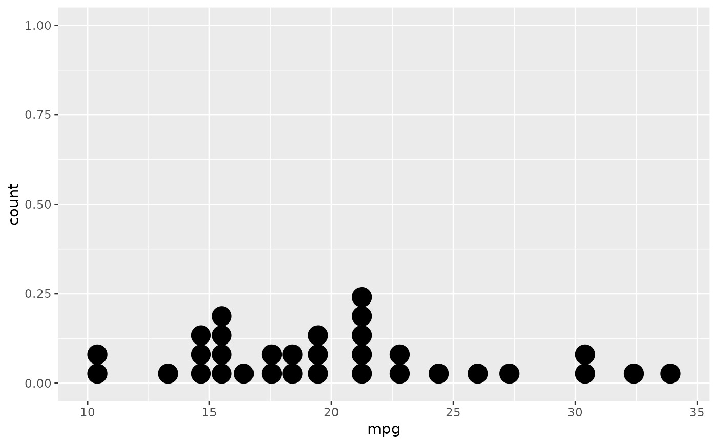
ggplot(mtcars, aes(x = mpg)) +
geom_dotplot()
#> Bin width defaults to 1/30 of the range of the data. Pick better value
#> with `binwidth`.
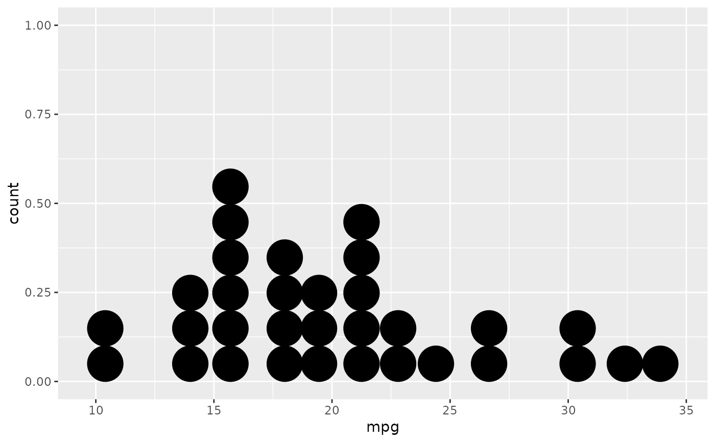
 ggplot(mtcars, aes(x = mpg)) +
geom_dotplot(binwidth = 1.5)
ggplot(mtcars, aes(x = mpg)) +
geom_dotplot(binwidth = 1.5)
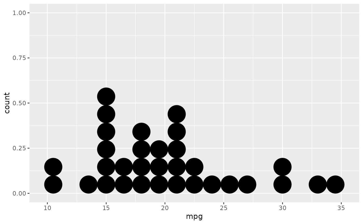
 # Use fixed-width bins
ggplot(mtcars, aes(x = mpg)) +
geom_dotplot(method="histodot", binwidth = 1.5)
# Use fixed-width bins
ggplot(mtcars, aes(x = mpg)) +
geom_dotplot(method="histodot", binwidth = 1.5)
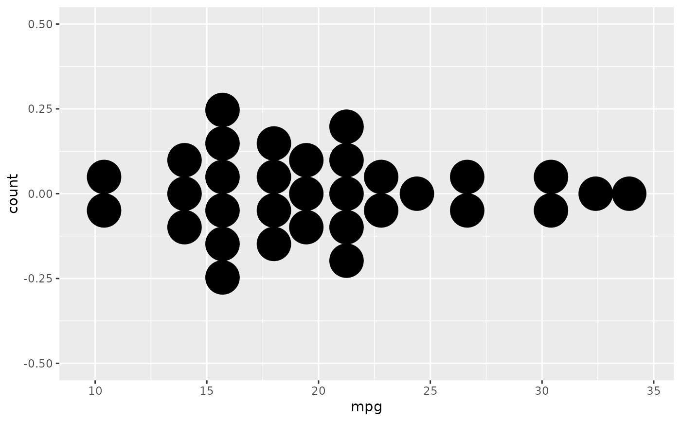
 # Some other stacking methods
ggplot(mtcars, aes(x = mpg)) +
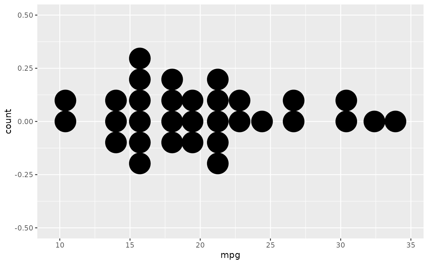
geom_dotplot(binwidth = 1.5, stackdir = "center")
# Some other stacking methods
ggplot(mtcars, aes(x = mpg)) +
geom_dotplot(binwidth = 1.5, stackdir = "center")
 ggplot(mtcars, aes(x = mpg)) +
geom_dotplot(binwidth = 1.5, stackdir = "centerwhole")
ggplot(mtcars, aes(x = mpg)) +
geom_dotplot(binwidth = 1.5, stackdir = "centerwhole")
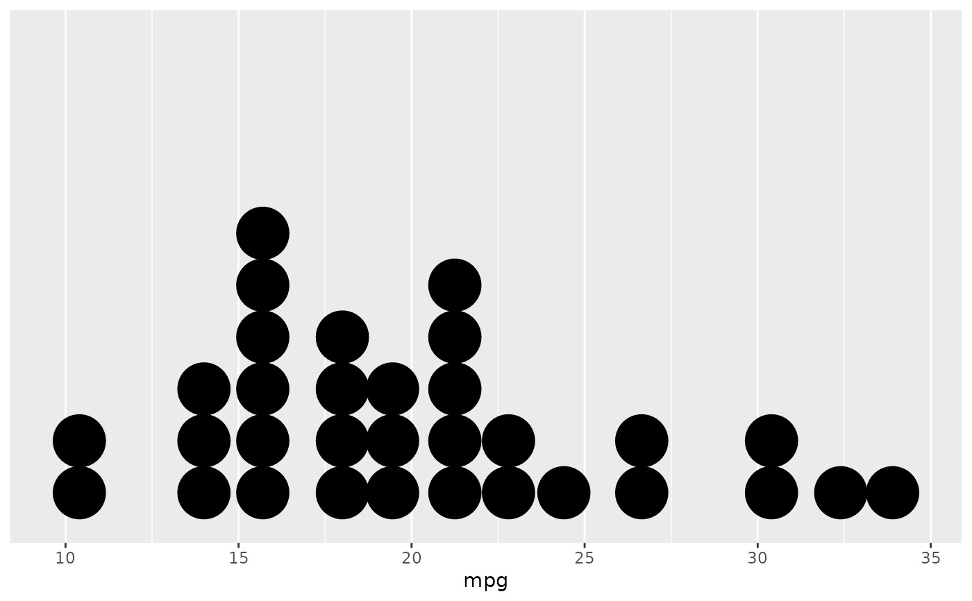
 # y axis isn't really meaningful, so hide it
ggplot(mtcars, aes(x = mpg)) + geom_dotplot(binwidth = 1.5) +
scale_y_continuous(NULL, breaks = NULL)
# y axis isn't really meaningful, so hide it
ggplot(mtcars, aes(x = mpg)) + geom_dotplot(binwidth = 1.5) +
scale_y_continuous(NULL, breaks = NULL)
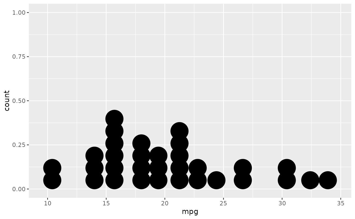
 # Overlap dots vertically
ggplot(mtcars, aes(x = mpg)) +
geom_dotplot(binwidth = 1.5, stackratio = .7)
# Overlap dots vertically
ggplot(mtcars, aes(x = mpg)) +
geom_dotplot(binwidth = 1.5, stackratio = .7)
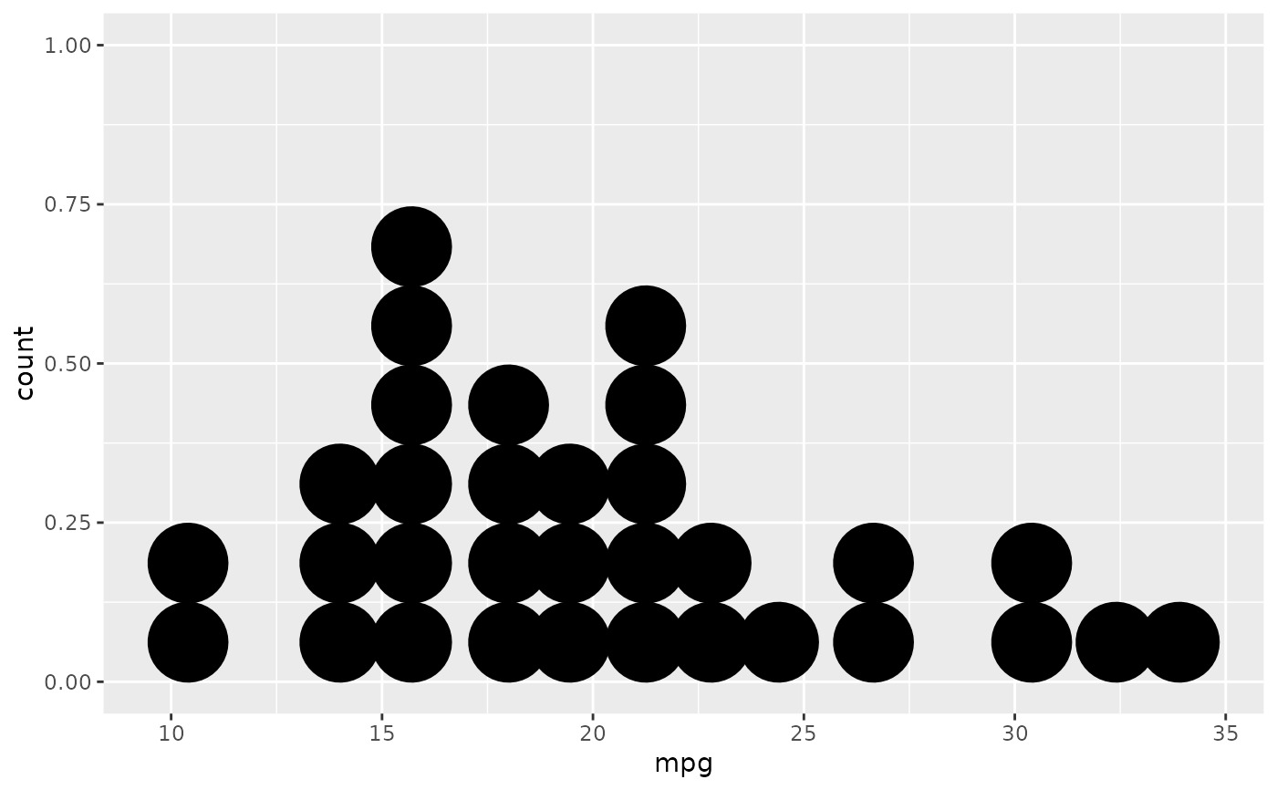
 # Expand dot diameter
ggplot(mtcars, aes(x = mpg)) +
geom_dotplot(binwidth = 1.5, dotsize = 1.25)
# Expand dot diameter
ggplot(mtcars, aes(x = mpg)) +
geom_dotplot(binwidth = 1.5, dotsize = 1.25)
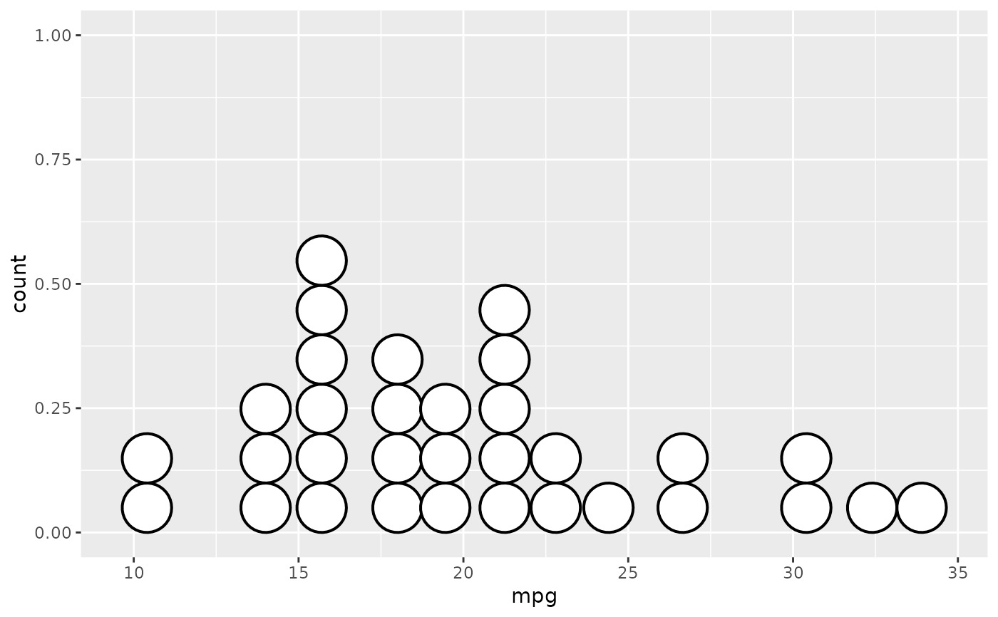
 # Change dot fill colour, stroke width
ggplot(mtcars, aes(x = mpg)) +
geom_dotplot(binwidth = 1.5, fill = "white", stroke = 2)
# Change dot fill colour, stroke width
ggplot(mtcars, aes(x = mpg)) +
geom_dotplot(binwidth = 1.5, fill = "white", stroke = 2)
 # \donttest{
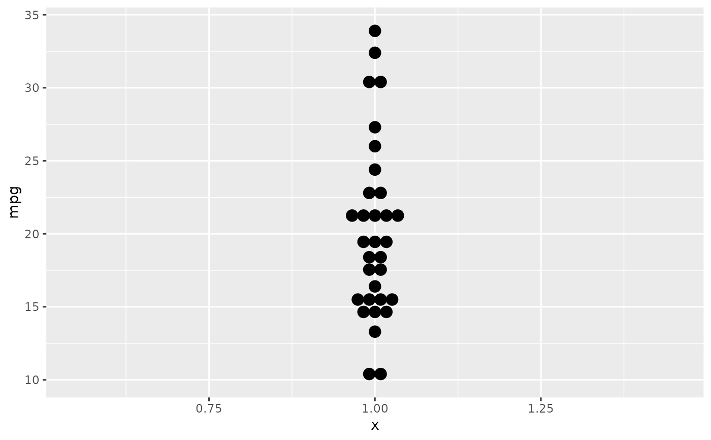
# Examples with stacking along y axis instead of x
ggplot(mtcars, aes(x = 1, y = mpg)) +
geom_dotplot(binaxis = "y", stackdir = "center")
#> Bin width defaults to 1/30 of the range of the data. Pick better value
#> with `binwidth`.
# \donttest{
# Examples with stacking along y axis instead of x
ggplot(mtcars, aes(x = 1, y = mpg)) +
geom_dotplot(binaxis = "y", stackdir = "center")
#> Bin width defaults to 1/30 of the range of the data. Pick better value
#> with `binwidth`.
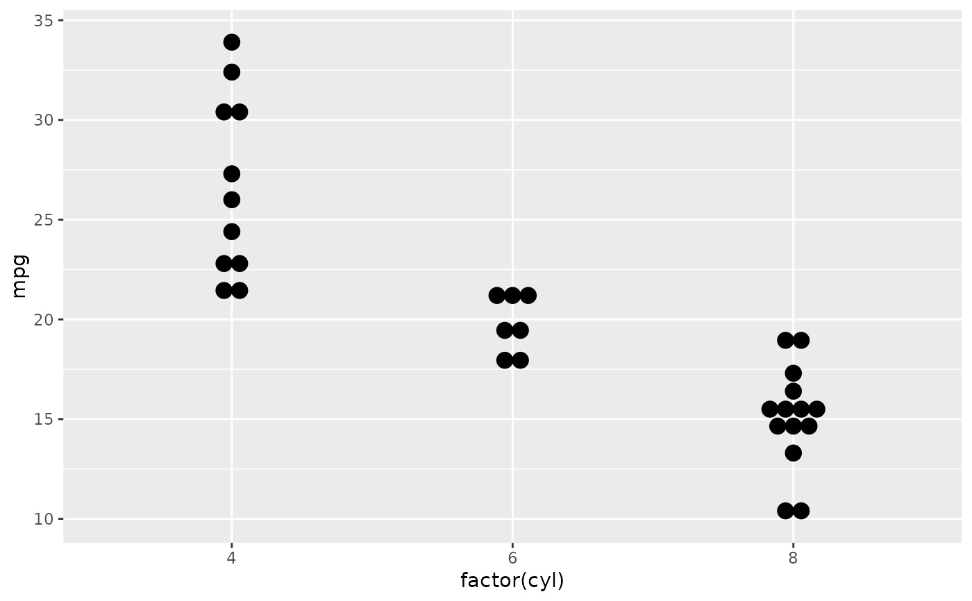
 ggplot(mtcars, aes(x = factor(cyl), y = mpg)) +
geom_dotplot(binaxis = "y", stackdir = "center")
#> Bin width defaults to 1/30 of the range of the data. Pick better value
#> with `binwidth`.
ggplot(mtcars, aes(x = factor(cyl), y = mpg)) +
geom_dotplot(binaxis = "y", stackdir = "center")
#> Bin width defaults to 1/30 of the range of the data. Pick better value
#> with `binwidth`.
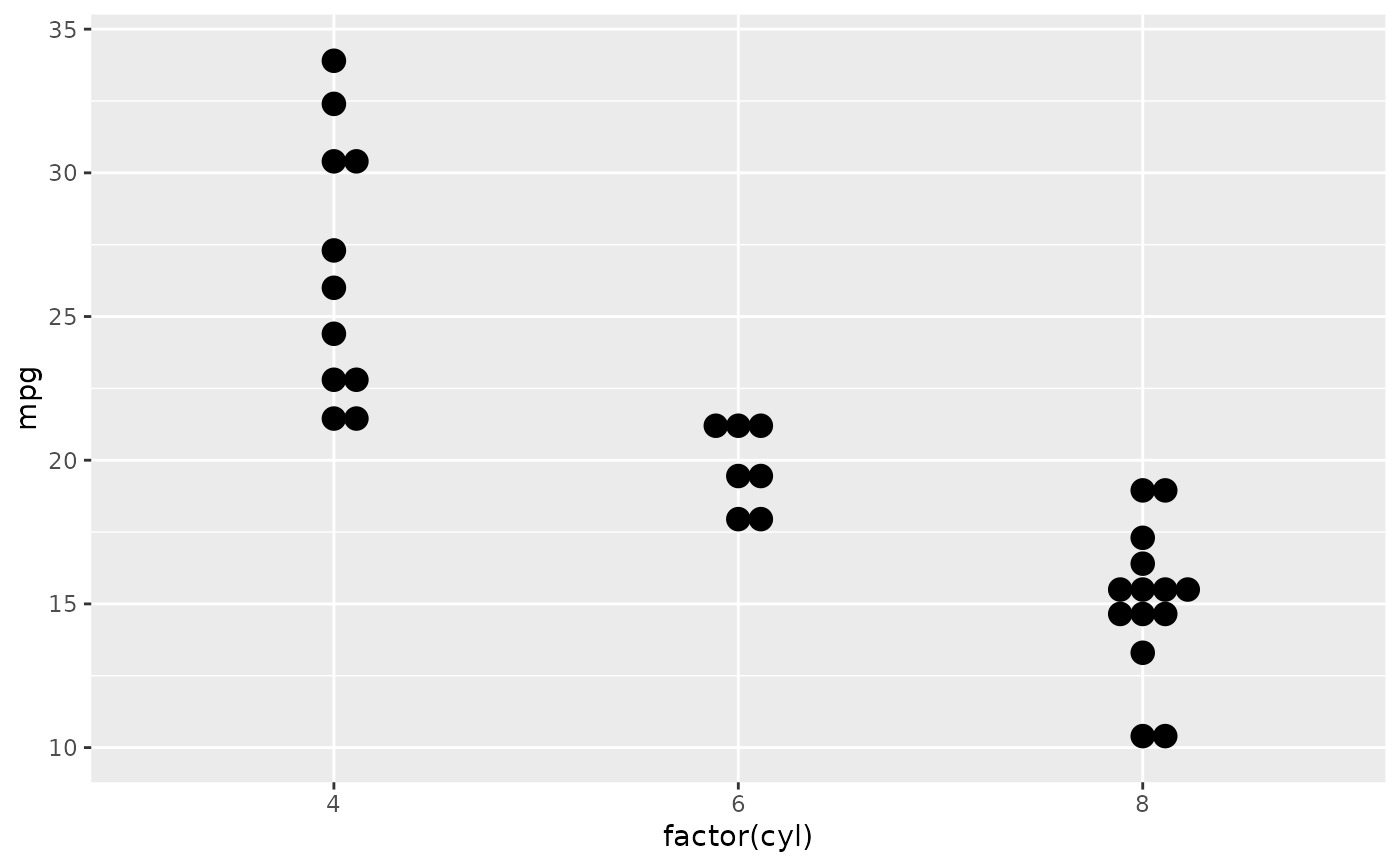
 ggplot(mtcars, aes(x = factor(cyl), y = mpg)) +
geom_dotplot(binaxis = "y", stackdir = "centerwhole")
#> Bin width defaults to 1/30 of the range of the data. Pick better value
#> with `binwidth`.
ggplot(mtcars, aes(x = factor(cyl), y = mpg)) +
geom_dotplot(binaxis = "y", stackdir = "centerwhole")
#> Bin width defaults to 1/30 of the range of the data. Pick better value
#> with `binwidth`.
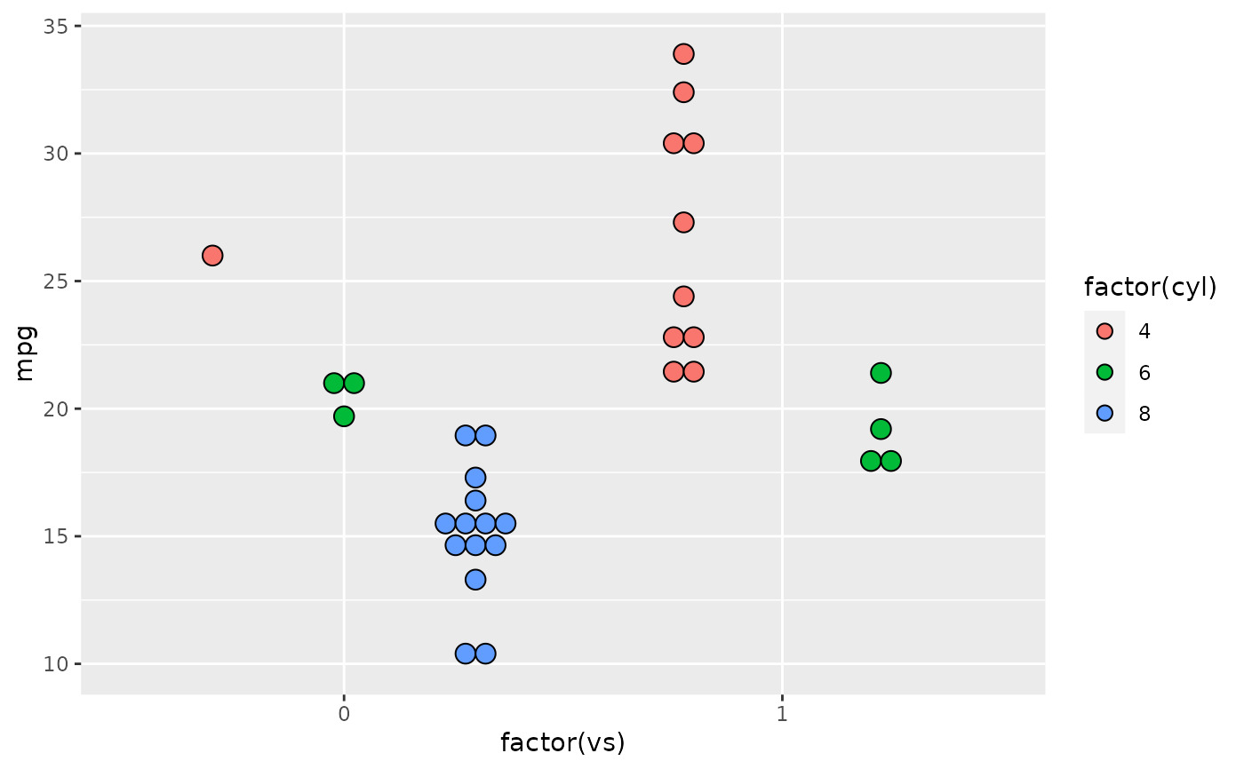
 ggplot(mtcars, aes(x = factor(vs), fill = factor(cyl), y = mpg)) +
geom_dotplot(binaxis = "y", stackdir = "center", position = "dodge")
#> Bin width defaults to 1/30 of the range of the data. Pick better value
#> with `binwidth`.
ggplot(mtcars, aes(x = factor(vs), fill = factor(cyl), y = mpg)) +
geom_dotplot(binaxis = "y", stackdir = "center", position = "dodge")
#> Bin width defaults to 1/30 of the range of the data. Pick better value
#> with `binwidth`.
 # binpositions="all" ensures that the bins are aligned between groups
ggplot(mtcars, aes(x = factor(am), y = mpg)) +
geom_dotplot(binaxis = "y", stackdir = "center", binpositions="all")
#> Bin width defaults to 1/30 of the range of the data. Pick better value
#> with `binwidth`.
# binpositions="all" ensures that the bins are aligned between groups
ggplot(mtcars, aes(x = factor(am), y = mpg)) +
geom_dotplot(binaxis = "y", stackdir = "center", binpositions="all")
#> Bin width defaults to 1/30 of the range of the data. Pick better value
#> with `binwidth`.
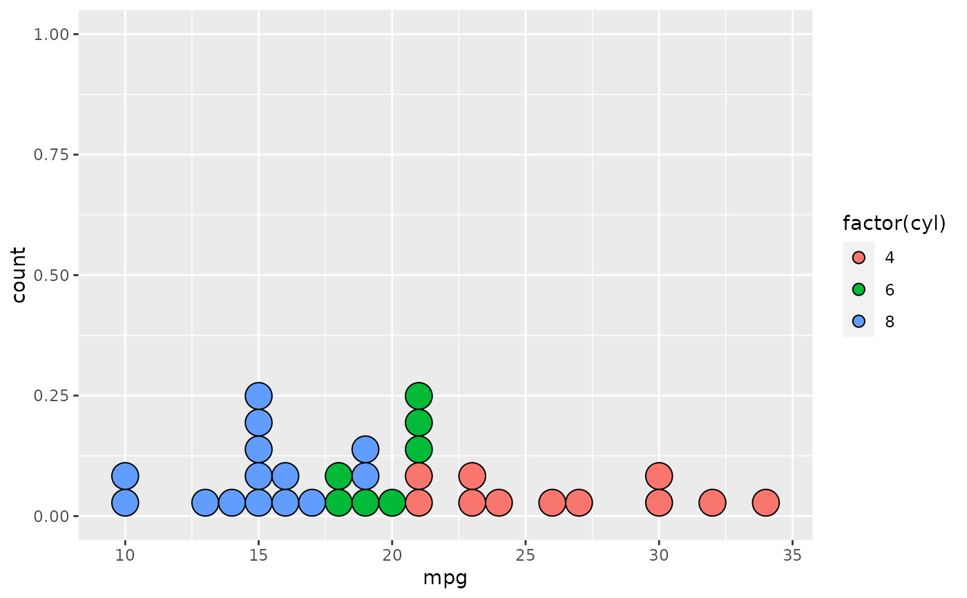
 # Stacking multiple groups, with different fill
ggplot(mtcars, aes(x = mpg, fill = factor(cyl))) +
geom_dotplot(stackgroups = TRUE, binwidth = 1, binpositions = "all")
# Stacking multiple groups, with different fill
ggplot(mtcars, aes(x = mpg, fill = factor(cyl))) +
geom_dotplot(stackgroups = TRUE, binwidth = 1, binpositions = "all")
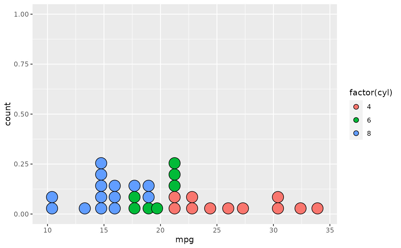 ggplot(mtcars, aes(x = mpg, fill = factor(cyl))) +
geom_dotplot(stackgroups = TRUE, binwidth = 1, method = "histodot")
ggplot(mtcars, aes(x = mpg, fill = factor(cyl))) +
geom_dotplot(stackgroups = TRUE, binwidth = 1, method = "histodot")
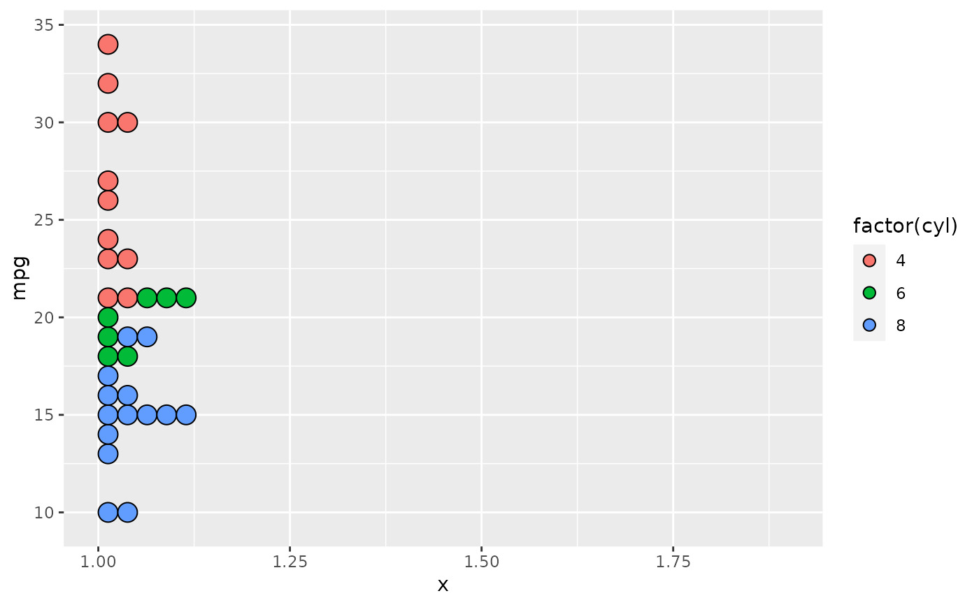
 ggplot(mtcars, aes(x = 1, y = mpg, fill = factor(cyl))) +
geom_dotplot(binaxis = "y", stackgroups = TRUE, binwidth = 1, method = "histodot")
ggplot(mtcars, aes(x = 1, y = mpg, fill = factor(cyl))) +
geom_dotplot(binaxis = "y", stackgroups = TRUE, binwidth = 1, method = "histodot")
 # }
# }
相關用法
- R ggplot2 geom_density_2d 二維密度估計的等值線
- R ggplot2 geom_density 平滑密度估計
- R ggplot2 geom_qq 分位數-分位數圖
- R ggplot2 geom_spoke 由位置、方向和距離參數化的線段
- R ggplot2 geom_quantile 分位數回歸
- R ggplot2 geom_text 文本
- R ggplot2 geom_ribbon 函數區和麵積圖
- R ggplot2 geom_boxplot 盒須圖(Tukey 風格)
- R ggplot2 geom_hex 二維箱計數的六邊形熱圖
- R ggplot2 geom_bar 條形圖
- R ggplot2 geom_bin_2d 二維 bin 計數熱圖
- R ggplot2 geom_jitter 抖動點
- R ggplot2 geom_point 積分
- R ggplot2 geom_linerange 垂直間隔:線、橫線和誤差線
- R ggplot2 geom_blank 什麽也不畫
- R ggplot2 geom_path 連接觀察結果
- R ggplot2 geom_violin 小提琴情節
- R ggplot2 geom_errorbarh 水平誤差線
- R ggplot2 geom_function 將函數繪製為連續曲線
- R ggplot2 geom_polygon 多邊形
- R ggplot2 geom_histogram 直方圖和頻數多邊形
- R ggplot2 geom_tile 矩形
- R ggplot2 geom_segment 線段和曲線
- R ggplot2 geom_map 參考Map中的多邊形
- R ggplot2 geom_abline 參考線:水平、垂直和對角線
注:本文由純淨天空篩選整理自Hadley Wickham等大神的英文原創作品 Dot plot。非經特殊聲明,原始代碼版權歸原作者所有,本譯文未經允許或授權,請勿轉載或複製。