多邊形與路徑(由 geom_path() 繪製)非常相似,隻是起點和終點是相連的,並且內部由 fill 著色。 group 美學決定了哪些案例連接在一起形成多邊形。從 R 3.6 及更高版本開始,可以通過提供子組美感來繪製帶孔的多邊形,該子組美感可將外環點與說明多邊形中的孔的點區分開來。
用法
geom_polygon(
  mapping = NULL,
  data = NULL,
  stat = "identity",
  position = "identity",
  rule = "evenodd",
  ...,
  na.rm = FALSE,
  show.legend = NA,
  inherit.aes = TRUE
)
參數
- mapping
-
由
aes()創建的一組美學映射。如果指定且inherit.aes = TRUE(默認),它將與繪圖頂層的默認映射組合。如果沒有繪圖映射,則必須提供mapping。 - data
-
該層要顯示的數據。有以下三種選擇:
如果默認為
NULL,則數據繼承自ggplot()調用中指定的繪圖數據。data.frame或其他對象將覆蓋繪圖數據。所有對象都將被強化以生成 DataFrame 。請參閱fortify()將為其創建變量。將使用單個參數(繪圖數據)調用
function。返回值必須是data.frame,並將用作圖層數據。可以從formula創建function(例如~ head(.x, 10))。 - stat
-
用於該層數據的統計變換,可以作為
ggprotoGeom子類,也可以作為命名去掉stat_前綴的統計數據的字符串(例如"count"而不是"stat_count") - position
-
位置調整,可以是命名調整的字符串(例如
"jitter"使用position_jitter),也可以是調用位置調整函數的結果。如果需要更改調整設置,請使用後者。 - rule
-
"evenodd"或"winding"。如果正在繪製帶孔的多邊形(使用subgroup美學),則此參數定義如何解釋孔坐標。有關說明,請參閱grid::pathGrob()中的示例。 - ...
-
其他參數傳遞給
layer()。這些通常是美學,用於將美學設置為固定值,例如colour = "red"或size = 3。它們也可能是配對的 geom/stat 的參數。 - na.rm
-
如果
FALSE,則默認缺失值將被刪除並帶有警告。如果TRUE,缺失值將被靜默刪除。 - show.legend
-
合乎邏輯的。該層是否應該包含在圖例中?
NA(默認值)包括是否映射了任何美學。FALSE從不包含,而TRUE始終包含。它也可以是一個命名的邏輯向量,以精細地選擇要顯示的美學。 - inherit.aes
-
如果
FALSE,則覆蓋默認美學,而不是與它們組合。這對於定義數據和美觀的輔助函數最有用,並且不應繼承默認繪圖規範的行為,例如borders()。
美學
geom_polygon() 理解以下美學(所需的美學以粗體顯示):
-
x -
y -
alpha -
colour -
fill -
group -
linetype -
linewidth -
subgroup
在 vignette("ggplot2-specs") 中了解有關設置這些美學的更多信息。
也可以看看
geom_path() 表示未填充的多邊形,geom_ribbon() 表示錨定在 x 軸上的多邊形
例子
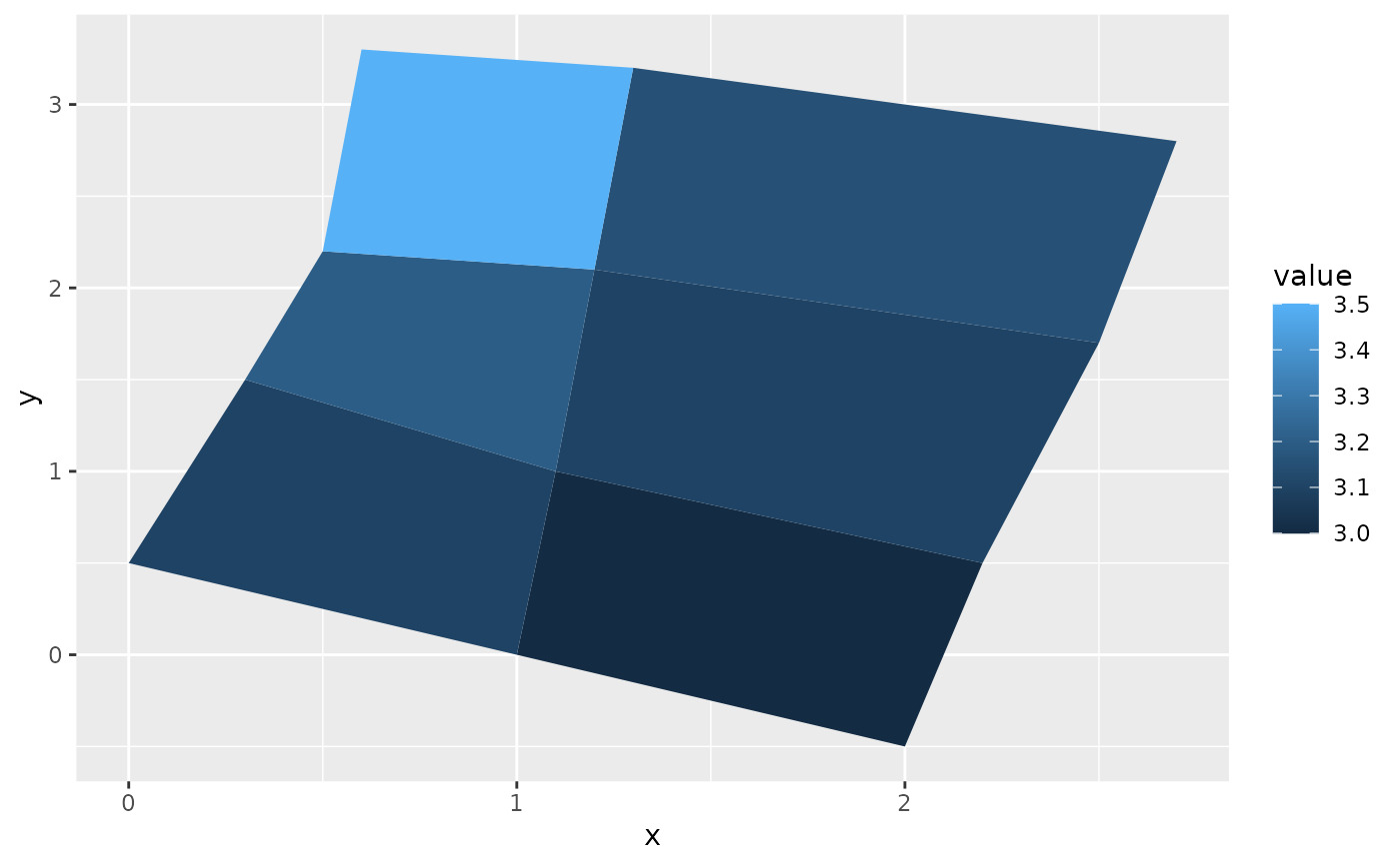
# When using geom_polygon, you will typically need two data frames:
# one contains the coordinates of each polygon (positions), and the
# other the values associated with each polygon (values). An id
# variable links the two together
ids <- factor(c("1.1", "2.1", "1.2", "2.2", "1.3", "2.3"))
values <- data.frame(
id = ids,
value = c(3, 3.1, 3.1, 3.2, 3.15, 3.5)
)
positions <- data.frame(
id = rep(ids, each = 4),
x = c(2, 1, 1.1, 2.2, 1, 0, 0.3, 1.1, 2.2, 1.1, 1.2, 2.5, 1.1, 0.3,
0.5, 1.2, 2.5, 1.2, 1.3, 2.7, 1.2, 0.5, 0.6, 1.3),
y = c(-0.5, 0, 1, 0.5, 0, 0.5, 1.5, 1, 0.5, 1, 2.1, 1.7, 1, 1.5,
2.2, 2.1, 1.7, 2.1, 3.2, 2.8, 2.1, 2.2, 3.3, 3.2)
)
# Currently we need to manually merge the two together
datapoly <- merge(values, positions, by = c("id"))
p <- ggplot(datapoly, aes(x = x, y = y)) +
geom_polygon(aes(fill = value, group = id))
p
 # Which seems like a lot of work, but then it's easy to add on
# other features in this coordinate system, e.g.:
set.seed(1)
stream <- data.frame(
x = cumsum(runif(50, max = 0.1)),
y = cumsum(runif(50,max = 0.1))
)
p + geom_line(data = stream, colour = "grey30", linewidth = 5)
# Which seems like a lot of work, but then it's easy to add on
# other features in this coordinate system, e.g.:
set.seed(1)
stream <- data.frame(
x = cumsum(runif(50, max = 0.1)),
y = cumsum(runif(50,max = 0.1))
)
p + geom_line(data = stream, colour = "grey30", linewidth = 5)
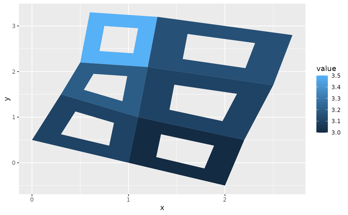
 # And if the positions are in longitude and latitude, you can use
# coord_map to produce different map projections.
if (packageVersion("grid") >= "3.6") {
# As of R version 3.6 geom_polygon() supports polygons with holes
# Use the subgroup aesthetic to differentiate holes from the main polygon
holes <- do.call(rbind, lapply(split(datapoly, datapoly$id), function(df) {
df$x <- df$x + 0.5 * (mean(df$x) - df$x)
df$y <- df$y + 0.5 * (mean(df$y) - df$y)
df
}))
datapoly$subid <- 1L
holes$subid <- 2L
datapoly <- rbind(datapoly, holes)
p <- ggplot(datapoly, aes(x = x, y = y)) +
geom_polygon(aes(fill = value, group = id, subgroup = subid))
p
}
# And if the positions are in longitude and latitude, you can use
# coord_map to produce different map projections.
if (packageVersion("grid") >= "3.6") {
# As of R version 3.6 geom_polygon() supports polygons with holes
# Use the subgroup aesthetic to differentiate holes from the main polygon
holes <- do.call(rbind, lapply(split(datapoly, datapoly$id), function(df) {
df$x <- df$x + 0.5 * (mean(df$x) - df$x)
df$y <- df$y + 0.5 * (mean(df$y) - df$y)
df
}))
datapoly$subid <- 1L
holes$subid <- 2L
datapoly <- rbind(datapoly, holes)
p <- ggplot(datapoly, aes(x = x, y = y)) +
geom_polygon(aes(fill = value, group = id, subgroup = subid))
p
}
相關用法
- R ggplot2 geom_point 積分
- R ggplot2 geom_path 連接觀察結果
- R ggplot2 geom_qq 分位數-分位數圖
- R ggplot2 geom_spoke 由位置、方向和距離參數化的線段
- R ggplot2 geom_quantile 分位數回歸
- R ggplot2 geom_text 文本
- R ggplot2 geom_ribbon 函數區和麵積圖
- R ggplot2 geom_boxplot 盒須圖(Tukey 風格)
- R ggplot2 geom_hex 二維箱計數的六邊形熱圖
- R ggplot2 geom_bar 條形圖
- R ggplot2 geom_bin_2d 二維 bin 計數熱圖
- R ggplot2 geom_jitter 抖動點
- R ggplot2 geom_linerange 垂直間隔:線、橫線和誤差線
- R ggplot2 geom_blank 什麽也不畫
- R ggplot2 geom_violin 小提琴情節
- R ggplot2 geom_dotplot 點圖
- R ggplot2 geom_errorbarh 水平誤差線
- R ggplot2 geom_function 將函數繪製為連續曲線
- R ggplot2 geom_histogram 直方圖和頻數多邊形
- R ggplot2 geom_tile 矩形
- R ggplot2 geom_segment 線段和曲線
- R ggplot2 geom_density_2d 二維密度估計的等值線
- R ggplot2 geom_map 參考Map中的多邊形
- R ggplot2 geom_density 平滑密度估計
- R ggplot2 geom_abline 參考線:水平、垂直和對角線
注:本文由純淨天空篩選整理自Hadley Wickham等大神的英文原創作品 Polygons。非經特殊聲明,原始代碼版權歸原作者所有,本譯文未經允許或授權,請勿轉載或複製。