這對數據進行分位數回歸擬合,並用線條繪製擬合的分位數。這是 geom_boxplot() 的連續模擬。
用法
geom_quantile(
  mapping = NULL,
  data = NULL,
  stat = "quantile",
  position = "identity",
  ...,
  lineend = "butt",
  linejoin = "round",
  linemitre = 10,
  na.rm = FALSE,
  show.legend = NA,
  inherit.aes = TRUE
)

stat_quantile(
  mapping = NULL,
  data = NULL,
  geom = "quantile",
  position = "identity",
  ...,
  quantiles = c(0.25, 0.5, 0.75),
  formula = NULL,
  method = "rq",
  method.args = list(),
  na.rm = FALSE,
  show.legend = NA,
  inherit.aes = TRUE
)
參數
- mapping
-
由
aes()創建的一組美學映射。如果指定且inherit.aes = TRUE(默認),它將與繪圖頂層的默認映射組合。如果沒有繪圖映射,則必須提供mapping。 - data
-
該層要顯示的數據。有以下三種選擇:
如果默認為
NULL,則數據繼承自ggplot()調用中指定的繪圖數據。data.frame或其他對象將覆蓋繪圖數據。所有對象都將被強化以生成 DataFrame 。請參閱fortify()將為其創建變量。將使用單個參數(繪圖數據)調用
function。返回值必須是data.frame,並將用作圖層數據。可以從formula創建function(例如~ head(.x, 10))。 - position
-
位置調整,可以是命名調整的字符串(例如
"jitter"使用position_jitter),也可以是調用位置調整函數的結果。如果需要更改調整設置,請使用後者。 - ...
-
其他參數傳遞給
layer()。這些通常是美學,用於將美學設置為固定值,例如colour = "red"或size = 3。它們也可能是配對的 geom/stat 的參數。 - lineend
-
線端樣式(圓形、對接、方形)。
- linejoin
-
線連接樣式(圓形、斜接、斜角)。
- linemitre
-
線斜接限製(數量大於 1)。
- na.rm
-
如果
FALSE,則默認缺失值將被刪除並帶有警告。如果TRUE,缺失值將被靜默刪除。 - show.legend
-
合乎邏輯的。該層是否應該包含在圖例中?
NA(默認值)包括是否映射了任何美學。FALSE從不包含,而TRUE始終包含。它也可以是一個命名的邏輯向量,以精細地選擇要顯示的美學。 - inherit.aes
-
如果
FALSE,則覆蓋默認美學,而不是與它們組合。這對於定義數據和美觀的輔助函數最有用,並且不應繼承默認繪圖規範的行為,例如borders()。 - geom, stat
-
用於覆蓋
geom_quantile()和stat_quantile()之間的默認連接。 - quantiles
-
要計算和顯示的 y 的條件分位數
- formula
-
將 y 變量與 x 變量相關的公式
- method
-
使用分位數回歸方法。可用選項為
"rq"(對於quantreg::rq())和"rqss"(對於quantreg::rqss())。 - method.args
-
傳遞給
method定義的建模函數的附加參數列表。
美學
geom_quantile() 理解以下美學(所需的美學以粗體顯示):
-
x -
y -
alpha -
colour -
group -
linetype -
linewidth -
weight
在 vignette("ggplot2-specs") 中了解有關設置這些美學的更多信息。
例子
m <-
ggplot(mpg, aes(displ, 1 / hwy)) +
geom_point()
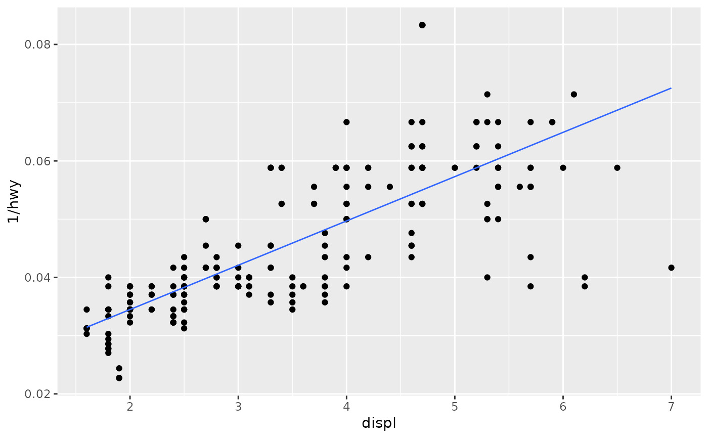
m + geom_quantile()
#> Smoothing formula not specified. Using: y ~ x
 m + geom_quantile(quantiles = 0.5)
#> Smoothing formula not specified. Using: y ~ x
m + geom_quantile(quantiles = 0.5)
#> Smoothing formula not specified. Using: y ~ x
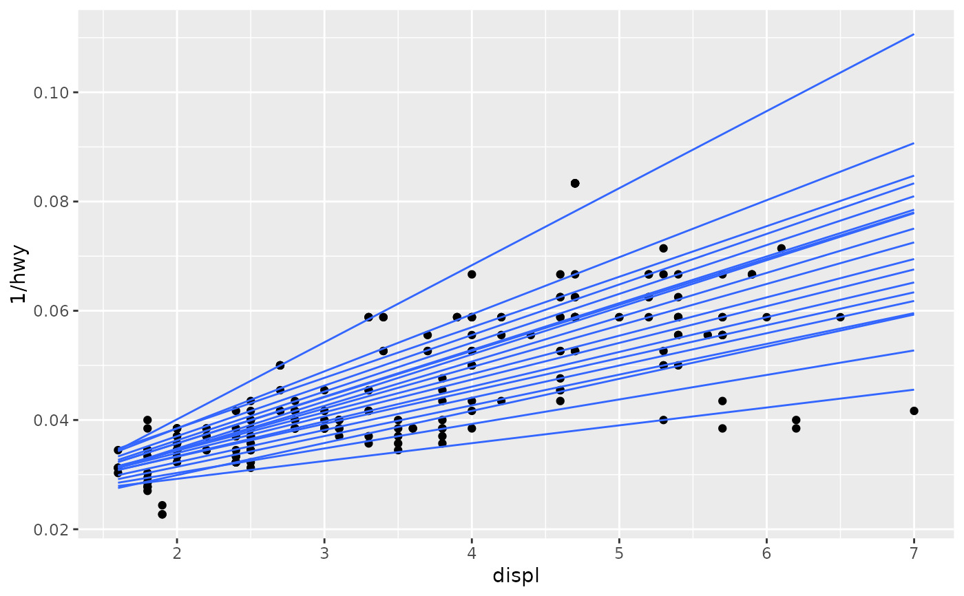
 q10 <- seq(0.05, 0.95, by = 0.05)
m + geom_quantile(quantiles = q10)
#> Smoothing formula not specified. Using: y ~ x
q10 <- seq(0.05, 0.95, by = 0.05)
m + geom_quantile(quantiles = q10)
#> Smoothing formula not specified. Using: y ~ x
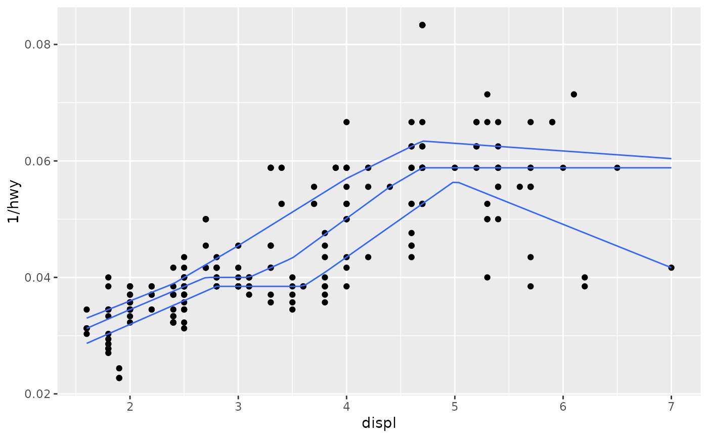
 # You can also use rqss to fit smooth quantiles
m + geom_quantile(method = "rqss")
#> Smoothing formula not specified. Using: y ~ qss(x, lambda = 1)
# You can also use rqss to fit smooth quantiles
m + geom_quantile(method = "rqss")
#> Smoothing formula not specified. Using: y ~ qss(x, lambda = 1)
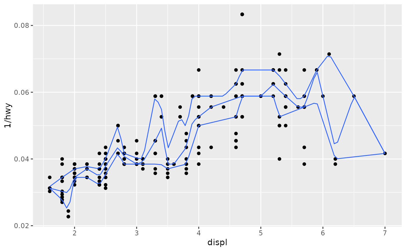
 # Note that rqss doesn't pick a smoothing constant automatically, so
# you'll need to tweak lambda yourself
m + geom_quantile(method = "rqss", lambda = 0.1)
#> Smoothing formula not specified. Using: y ~ qss(x, lambda = 0.1)
# Note that rqss doesn't pick a smoothing constant automatically, so
# you'll need to tweak lambda yourself
m + geom_quantile(method = "rqss", lambda = 0.1)
#> Smoothing formula not specified. Using: y ~ qss(x, lambda = 0.1)
 # Set aesthetics to fixed value
m + geom_quantile(colour = "red", linewidth = 2, alpha = 0.5)
#> Smoothing formula not specified. Using: y ~ x
# Set aesthetics to fixed value
m + geom_quantile(colour = "red", linewidth = 2, alpha = 0.5)
#> Smoothing formula not specified. Using: y ~ x

相關用法
- R ggplot2 geom_qq 分位數-分位數圖
- R ggplot2 geom_spoke 由位置、方向和距離參數化的線段
- R ggplot2 geom_text 文本
- R ggplot2 geom_ribbon 函數區和麵積圖
- R ggplot2 geom_boxplot 盒須圖(Tukey 風格)
- R ggplot2 geom_hex 二維箱計數的六邊形熱圖
- R ggplot2 geom_bar 條形圖
- R ggplot2 geom_bin_2d 二維 bin 計數熱圖
- R ggplot2 geom_jitter 抖動點
- R ggplot2 geom_point 積分
- R ggplot2 geom_linerange 垂直間隔:線、橫線和誤差線
- R ggplot2 geom_blank 什麽也不畫
- R ggplot2 geom_path 連接觀察結果
- R ggplot2 geom_violin 小提琴情節
- R ggplot2 geom_dotplot 點圖
- R ggplot2 geom_errorbarh 水平誤差線
- R ggplot2 geom_function 將函數繪製為連續曲線
- R ggplot2 geom_polygon 多邊形
- R ggplot2 geom_histogram 直方圖和頻數多邊形
- R ggplot2 geom_tile 矩形
- R ggplot2 geom_segment 線段和曲線
- R ggplot2 geom_density_2d 二維密度估計的等值線
- R ggplot2 geom_map 參考Map中的多邊形
- R ggplot2 geom_density 平滑密度估計
- R ggplot2 geom_abline 參考線:水平、垂直和對角線
注:本文由純淨天空篩選整理自Hadley Wickham等大神的英文原創作品 Quantile regression。非經特殊聲明,原始代碼版權歸原作者所有,本譯文未經允許或授權,請勿轉載或複製。