R ggplot2 geom_segment 線段和曲線

geom_segment() 在點 (x, y) 和 (xend, Yend) 之間繪製一條直線。 geom_curve() 繪製一條曲線。有關控製曲線的參數，請參閱底層繪圖函數grid::curveGrob()。

用法

geom_segment(
  mapping = NULL,
  data = NULL,
  stat = "identity",
  position = "identity",
  ...,
  arrow = NULL,
  arrow.fill = NULL,
  lineend = "butt",
  linejoin = "round",
  na.rm = FALSE,
  show.legend = NA,
  inherit.aes = TRUE
)

geom_curve(
  mapping = NULL,
  data = NULL,
  stat = "identity",
  position = "identity",
  ...,
  curvature = 0.5,
  angle = 90,
  ncp = 5,
  arrow = NULL,
  arrow.fill = NULL,
  lineend = "butt",
  na.rm = FALSE,
  show.legend = NA,
  inherit.aes = TRUE
)

參數

mapping

由 aes() 創建的一組美學映射。如果指定且inherit.aes = TRUE(默認)，它將與繪圖頂層的默認映射組合。如果沒有繪圖映射，則必須提供mapping。

data

該層要顯示的數據。有以下三種選擇：

如果默認為 NULL ，則數據繼承自 ggplot() 調用中指定的繪圖數據。

data.frame 或其他對象將覆蓋繪圖數據。所有對象都將被強化以生成 DataFrame 。請參閱fortify() 將為其創建變量。

將使用單個參數(繪圖數據)調用function。返回值必須是 data.frame ，並將用作圖層數據。可以從 formula 創建 function (例如 ~ head(.x, 10) )。

stat

用於該層數據的統計變換，可以作為 ggproto Geom 子類，也可以作為命名去掉 stat_ 前綴的統計數據的字符串(例如 "count" 而不是 "stat_count" )

position

位置調整，可以是命名調整的字符串(例如 "jitter" 使用 position_jitter )，也可以是調用位置調整函數的結果。如果需要更改調整設置，請使用後者。

...

其他參數傳遞給 layer() 。這些通常是美學，用於將美學設置為固定值，例如 colour = "red" 或 size = 3 。它們也可能是配對的 geom/stat 的參數。

arrow

箭頭規範，由 grid::arrow() 創建。

arrow.fill

用於箭頭的填充顏色(如果關閉)。 NULL意味著使用colour美學。

lineend

線端樣式(圓形、對接、方形)。

linejoin

線連接樣式(圓形、斜接、斜角)。

na.rm

如果 FALSE ，則默認缺失值將被刪除並帶有警告。如果 TRUE ，缺失值將被靜默刪除。

show.legend

合乎邏輯的。該層是否應該包含在圖例中？ NA(默認值)包括是否映射了任何美學。 FALSE 從不包含，而 TRUE 始終包含。它也可以是一個命名的邏輯向量，以精細地選擇要顯示的美學。

inherit.aes

如果 FALSE ，則覆蓋默認美學，而不是與它們組合。這對於定義數據和美觀的輔助函數最有用，並且不應繼承默認繪圖規範的行為，例如borders() 。

curvature

給出曲率量的數值。負值產生左手曲線，正值產生右手曲線，零產生直線。

angle

0 到 180 之間的數值，給出曲線控製點的傾斜量。小於 90 的值使曲線向起點傾斜，大於 90 的值使曲線向終點傾斜。

ncp

用於繪製曲線的控製點的數量。更多控製點可創建更平滑的曲線。

細節

兩種幾何圖形都為每種情況繪製一條線段/曲線。如果您需要跨多個案例連接點，請參閱geom_path()。

美學

geom_segment() 理解以下美學(所需的美學以粗體顯示)：

x
y
xend
yend
alpha
colour
group
linetype
linewidth

在 vignette("ggplot2-specs") 中了解有關設置這些美學的更多信息。

也可以看看

geom_path() 和 geom_line() 用於多段線和路徑。

geom_spoke() 用於由位置 (x, y) 以及角度和半徑參數化的線段。

例子

b <- ggplot(mtcars, aes(wt, mpg)) +
  geom_point()

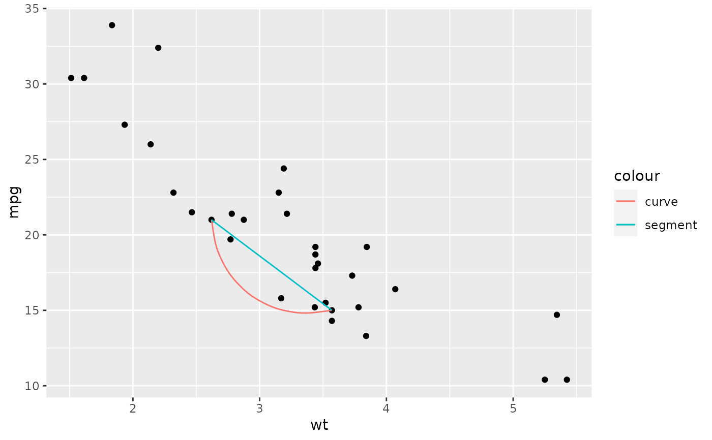
df <- data.frame(x1 = 2.62, x2 = 3.57, y1 = 21.0, y2 = 15.0)
b +
 geom_curve(aes(x = x1, y = y1, xend = x2, yend = y2, colour = "curve"), data = df) +
 geom_segment(aes(x = x1, y = y1, xend = x2, yend = y2, colour = "segment"), data = df)


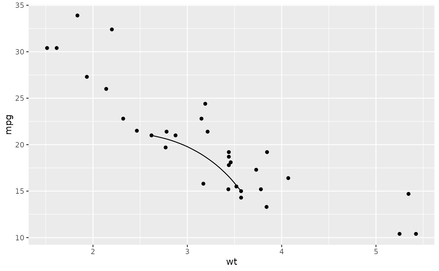
b + geom_curve(aes(x = x1, y = y1, xend = x2, yend = y2), data = df, curvature = -0.2)

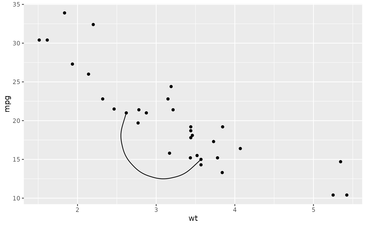
b + geom_curve(aes(x = x1, y = y1, xend = x2, yend = y2), data = df, curvature = 1)

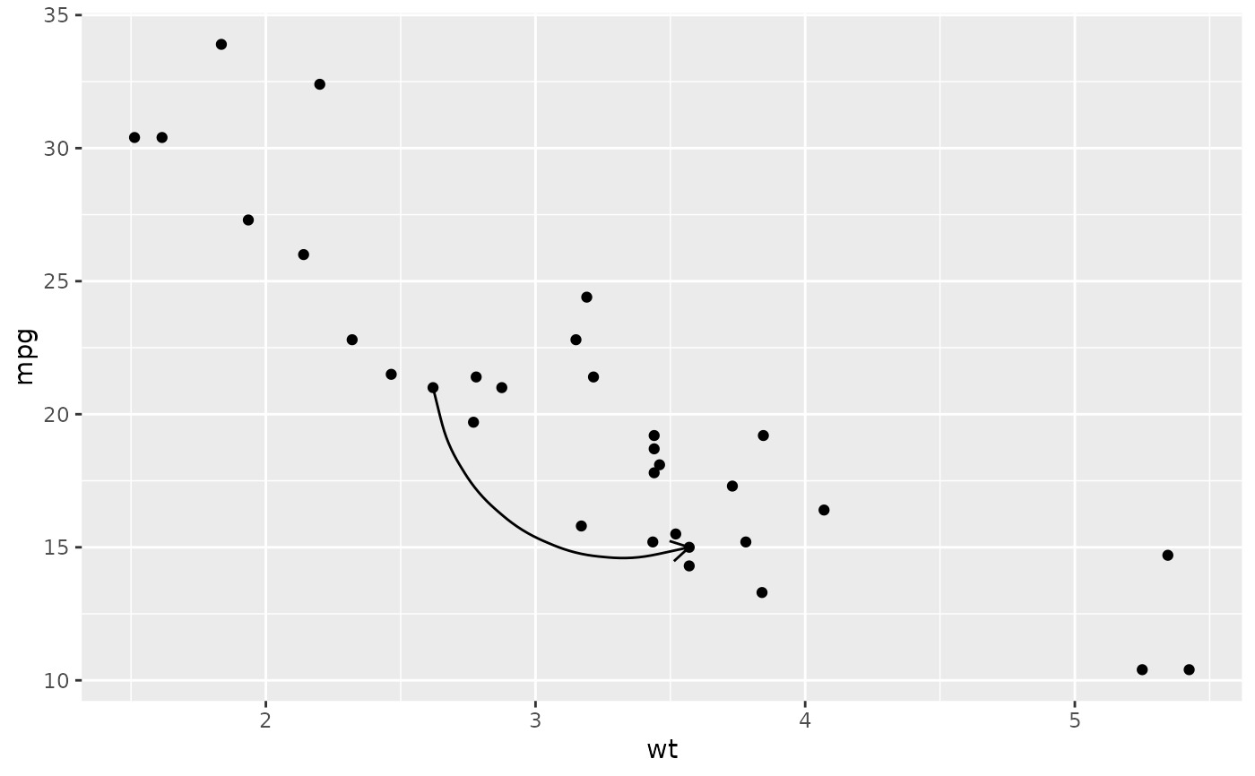
b + geom_curve(
  aes(x = x1, y = y1, xend = x2, yend = y2),
  data = df,
  arrow = arrow(length = unit(0.03, "npc"))
)


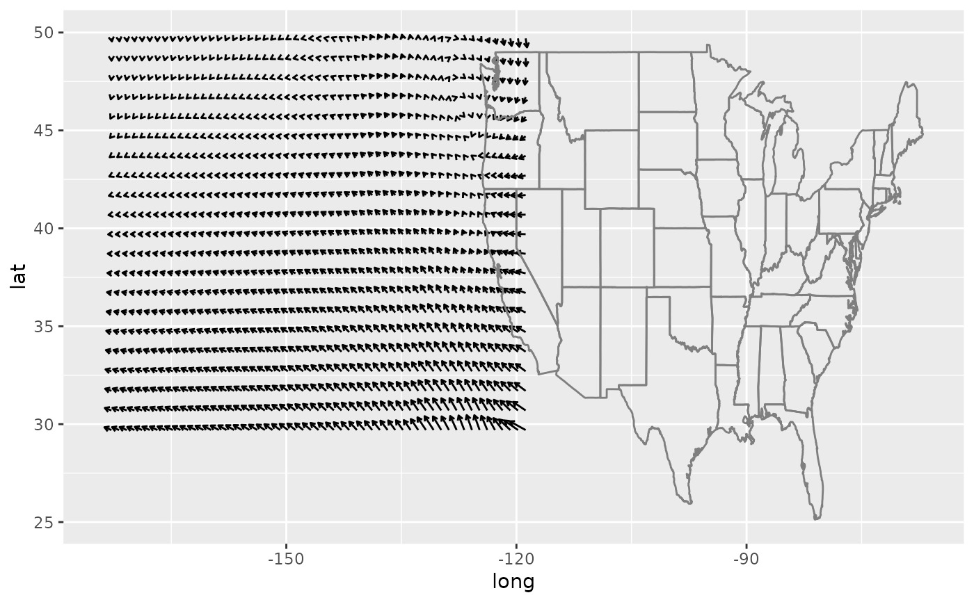
if (requireNamespace('maps', quietly = TRUE)) {
ggplot(seals, aes(long, lat)) +
  geom_segment(aes(xend = long + delta_long, yend = lat + delta_lat),
    arrow = arrow(length = unit(0.1,"cm"))) +
  borders("state")
}


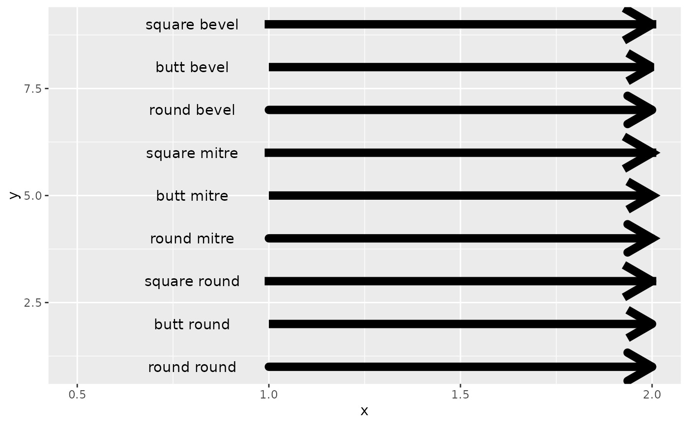
# Use lineend and linejoin to change the style of the segments
df2 <- expand.grid(
  lineend = c('round', 'butt', 'square'),
  linejoin = c('round', 'mitre', 'bevel'),
  stringsAsFactors = FALSE
)
df2 <- data.frame(df2, y = 1:9)
ggplot(df2, aes(x = 1, y = y, xend = 2, yend = y, label = paste(lineend, linejoin))) +
  geom_segment(
     lineend = df2$lineend, linejoin = df2$linejoin,
     size = 3, arrow = arrow(length = unit(0.3, "inches"))
  ) +
  geom_text(hjust = 'outside', nudge_x = -0.2) +
  xlim(0.5, 2)


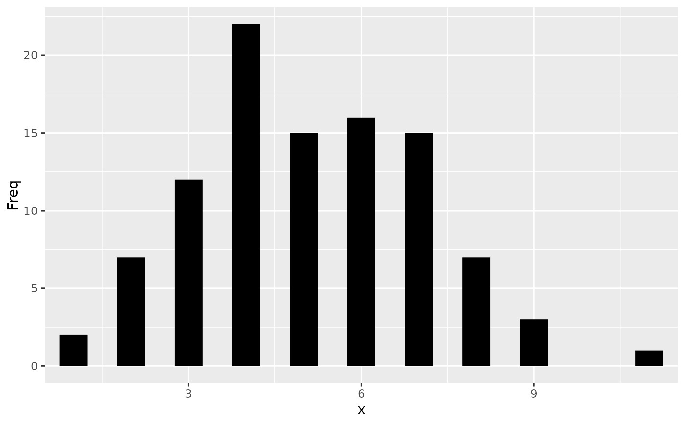
# You can also use geom_segment to recreate plot(type = "h") :
set.seed(1)
counts <- as.data.frame(table(x = rpois(100,5)))
counts$x <- as.numeric(as.character(counts$x))
with(counts, plot(x, Freq, type = "h", lwd = 10))


ggplot(counts, aes(x, Freq)) +
  geom_segment(aes(xend = x, yend = 0), linewidth = 10, lineend = "butt")

源代碼：R/geom-segment.R、R/geom-curve.R

相關用法

注：本文由純淨天空篩選整理自Hadley Wickham等大神的英文原創作品 Line segments and curves。非經特殊聲明，原始代碼版權歸原作者所有，本譯文未經允許或授權，請勿轉載或複製。