幫助眼睛在存在過度繪製的情況下看到模式。 geom_smooth() 和 stat_smooth() 實際上是別名:它們都使用相同的參數。如果要使用非標準幾何圖形顯示結果,請使用stat_smooth()。
用法
geom_smooth(
  mapping = NULL,
  data = NULL,
  stat = "smooth",
  position = "identity",
  ...,
  method = NULL,
  formula = NULL,
  se = TRUE,
  na.rm = FALSE,
  orientation = NA,
  show.legend = NA,
  inherit.aes = TRUE
)

stat_smooth(
  mapping = NULL,
  data = NULL,
  geom = "smooth",
  position = "identity",
  ...,
  method = NULL,
  formula = NULL,
  se = TRUE,
  n = 80,
  span = 0.75,
  fullrange = FALSE,
  level = 0.95,
  method.args = list(),
  na.rm = FALSE,
  orientation = NA,
  show.legend = NA,
  inherit.aes = TRUE
)
參數
- mapping
-
由
aes()創建的一組美學映射。如果指定且inherit.aes = TRUE(默認),它將與繪圖頂層的默認映射組合。如果沒有繪圖映射,則必須提供mapping。 - data
-
該層要顯示的數據。有以下三種選擇:
如果默認為
NULL,則數據繼承自ggplot()調用中指定的繪圖數據。data.frame或其他對象將覆蓋繪圖數據。所有對象都將被強化以生成 DataFrame 。請參閱fortify()將為其創建變量。將使用單個參數(繪圖數據)調用
function。返回值必須是data.frame,並將用作圖層數據。可以從formula創建function(例如~ head(.x, 10))。 - position
-
位置調整,可以是命名調整的字符串(例如
"jitter"使用position_jitter),也可以是調用位置調整函數的結果。如果需要更改調整設置,請使用後者。 - ...
-
其他參數傳遞給
layer()。這些通常是美學,用於將美學設置為固定值,例如colour = "red"或size = 3。它們也可能是配對的 geom/stat 的參數。 - method
-
要使用的平滑方法(函數)接受
NULL或字符向量,例如"lm"、"glm"、"gam"、"loess"或函數,例如MASS::rlm或mgcv::gam、stats::lm或stats::loess。為了向後兼容,"auto"也被接受。它相當於NULL。對於
method = NULL,平滑方法是根據最大組的大小(跨所有麵板)選擇的。stats::loess()用於少於 1,000 個觀測值;否則mgcv::gam()與formula = y ~ s(x, bs = "cs")和method = "REML"一起使用。有趣的是,loess提供了更好的外觀,但在內存中是 \(O(N^{2})\),因此不適用於較大的數據集。如果您的觀測值少於 1,000 個,但想要使用與
method = NULL相同的gam()模型,則設置method = "gam", formula = y ~ s(x, bs = "cs")。 - formula
-
用於平滑函數的公式,例如
y ~ x、y ~ poly(x, 2)、y ~ log(x)。默認情況下NULL,在這種情況下,當觀測值少於 1,000 個時,method = NULL意味著formula = y ~ x,否則formula = y ~ s(x, bs = "cs")。 - se
-
顯示平滑周圍的置信區間? (默認為
TRUE,參見level進行控製。) - na.rm
-
如果
FALSE,則默認缺失值將被刪除並帶有警告。如果TRUE,缺失值將被靜默刪除。 - orientation
-
層的方向。默認值 (
NA) 自動根據美學映射確定方向。萬一失敗,可以通過將orientation設置為"x"或"y"來顯式給出。有關更多詳細信息,請參閱方向部分。 - show.legend
-
合乎邏輯的。該層是否應該包含在圖例中?
NA(默認值)包括是否映射了任何美學。FALSE從不包含,而TRUE始終包含。它也可以是一個命名的邏輯向量,以精細地選擇要顯示的美學。 - inherit.aes
-
如果
FALSE,則覆蓋默認美學,而不是與它們組合。這對於定義數據和美觀的輔助函數最有用,並且不應繼承默認繪圖規範的行為,例如borders()。 - geom, stat
-
用於覆蓋
geom_smooth()和stat_smooth()之間的默認連接。 - n
-
評估更平滑的點數。
- span
-
控製默認 loess 平滑器的平滑量。較小的數字產生較彎曲的線條,較大的數字產生較平滑的線條。僅與黃土一起使用,即當
method = "loess"或method = NULL(默認)且觀測值少於 1,000 個時。 - fullrange
-
如果
TRUE,平滑線將擴展到繪圖範圍,可能超出數據範圍。這不會將該行擴展到expansion創建的任何附加填充中。 - level
-
要使用的置信區間水平(默認為 0.95)。
- method.args
-
傳遞給
method定義的建模函數的附加參數列表。
細節
計算由(當前未記錄的)predictdf() 泛型及其方法執行。對於大多數方法,標準誤差界限是使用 predict() 方法計算的 - 例外是 loess() ,它使用基於 t 的近似,以及 glm() ,其中正常置信區間是在鏈接尺度上構造的,然後back-transformed 到響應量表。
方向
該幾何體以不同的方式對待每個軸,因此可以有兩個方向。通常,方向很容易從給定映射和使用的位置比例類型的組合中推斷出來。因此,ggplot2 默認情況下會嘗試猜測圖層應具有哪個方向。在極少數情況下,方向不明確,猜測可能會失敗。在這種情況下,可以直接使用 orientation 參數指定方向,該參數可以是 "x" 或 "y" 。該值給出了幾何圖形應沿著的軸,"x" 是您期望的幾何圖形的默認方向。
美學
geom_smooth() 理解以下美學(所需的美學以粗體顯示):
-
x -
y -
alpha -
colour -
fill -
group -
linetype -
linewidth -
weight -
ymax -
ymin
在 vignette("ggplot2-specs") 中了解有關設置這些美學的更多信息。
計算變量
這些是由層的 'stat' 部分計算的,可以使用 delayed evaluation 訪問。 stat_smooth() 提供以下變量,其中一些取決於方向:
-
after_stat(y)或者after_stat(x)
預測值。 -
after_stat(ymin)或者after_stat(xmin)
均值附近逐點置信區間較低。 -
after_stat(ymax)或者after_stat(xmax)
均值周圍逐點置信區間的上限。 -
after_stat(se)
標準誤差。
例子
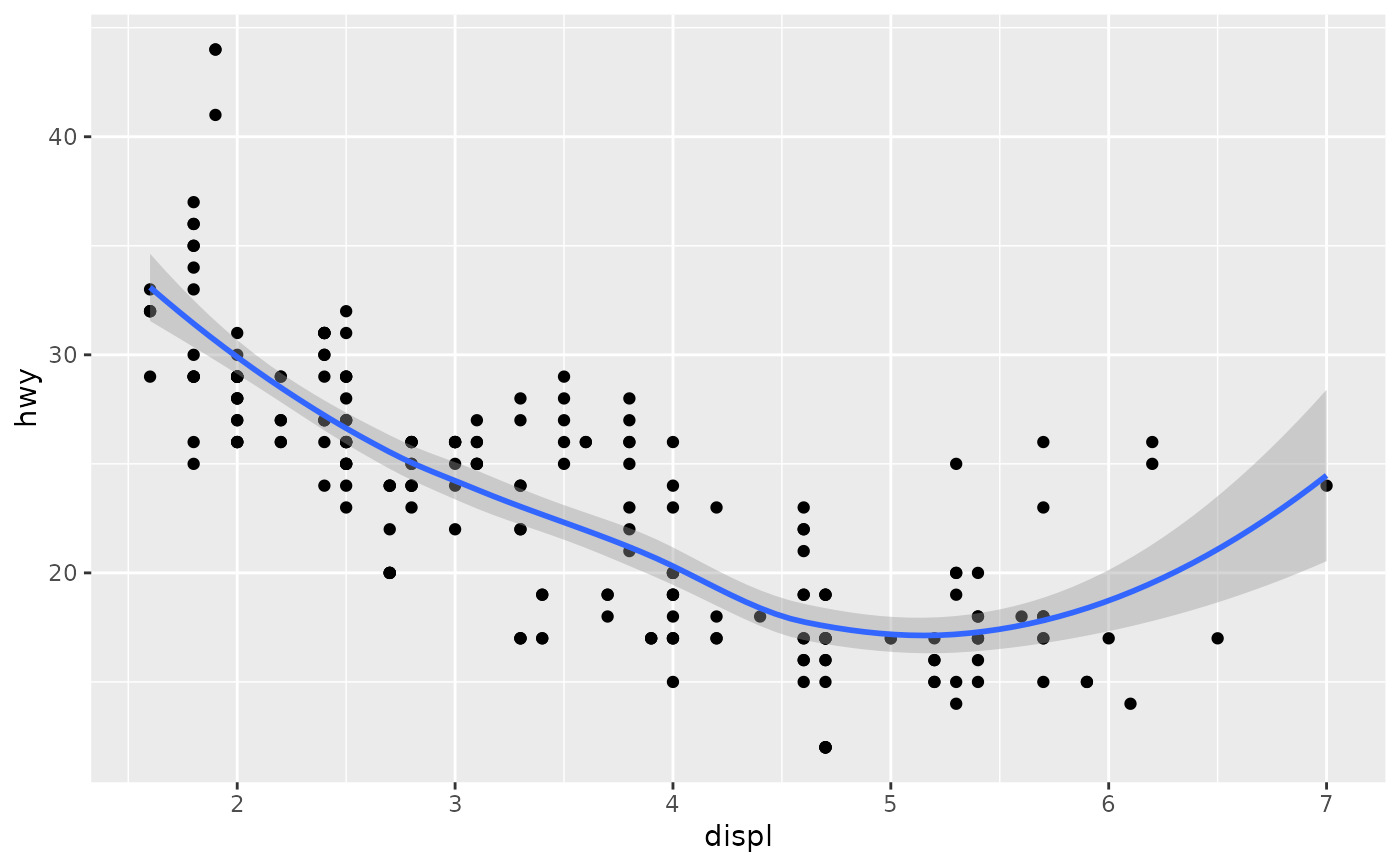
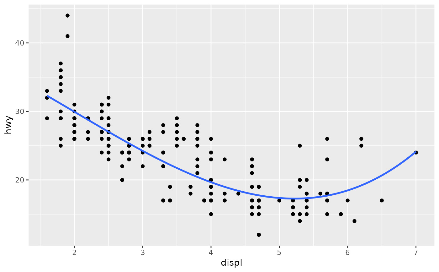
ggplot(mpg, aes(displ, hwy)) +
geom_point() +
geom_smooth()
#> `geom_smooth()` using method = 'loess' and formula = 'y ~ x'
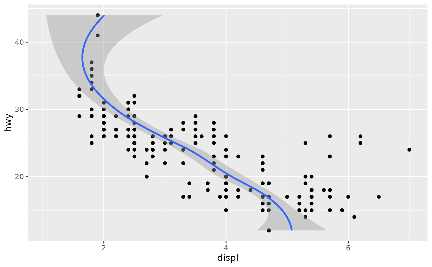
 # If you need the fitting to be done along the y-axis set the orientation
ggplot(mpg, aes(displ, hwy)) +
geom_point() +
geom_smooth(orientation = "y")
#> `geom_smooth()` using method = 'loess' and formula = 'y ~ x'
# If you need the fitting to be done along the y-axis set the orientation
ggplot(mpg, aes(displ, hwy)) +
geom_point() +
geom_smooth(orientation = "y")
#> `geom_smooth()` using method = 'loess' and formula = 'y ~ x'
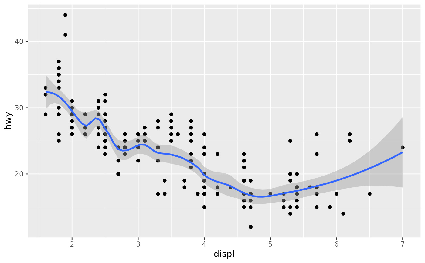
 # Use span to control the "wiggliness" of the default loess smoother.
# The span is the fraction of points used to fit each local regression:
# small numbers make a wigglier curve, larger numbers make a smoother curve.
ggplot(mpg, aes(displ, hwy)) +
geom_point() +
geom_smooth(span = 0.3)
#> `geom_smooth()` using method = 'loess' and formula = 'y ~ x'
# Use span to control the "wiggliness" of the default loess smoother.
# The span is the fraction of points used to fit each local regression:
# small numbers make a wigglier curve, larger numbers make a smoother curve.
ggplot(mpg, aes(displ, hwy)) +
geom_point() +
geom_smooth(span = 0.3)
#> `geom_smooth()` using method = 'loess' and formula = 'y ~ x'
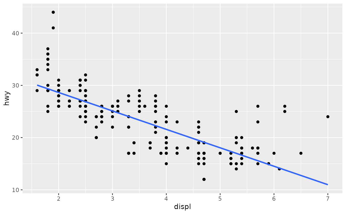
 # Instead of a loess smooth, you can use any other modelling function:
ggplot(mpg, aes(displ, hwy)) +
geom_point() +
geom_smooth(method = lm, se = FALSE)
#> `geom_smooth()` using formula = 'y ~ x'
# Instead of a loess smooth, you can use any other modelling function:
ggplot(mpg, aes(displ, hwy)) +
geom_point() +
geom_smooth(method = lm, se = FALSE)
#> `geom_smooth()` using formula = 'y ~ x'
 ggplot(mpg, aes(displ, hwy)) +
geom_point() +
geom_smooth(method = lm, formula = y ~ splines::bs(x, 3), se = FALSE)
ggplot(mpg, aes(displ, hwy)) +
geom_point() +
geom_smooth(method = lm, formula = y ~ splines::bs(x, 3), se = FALSE)
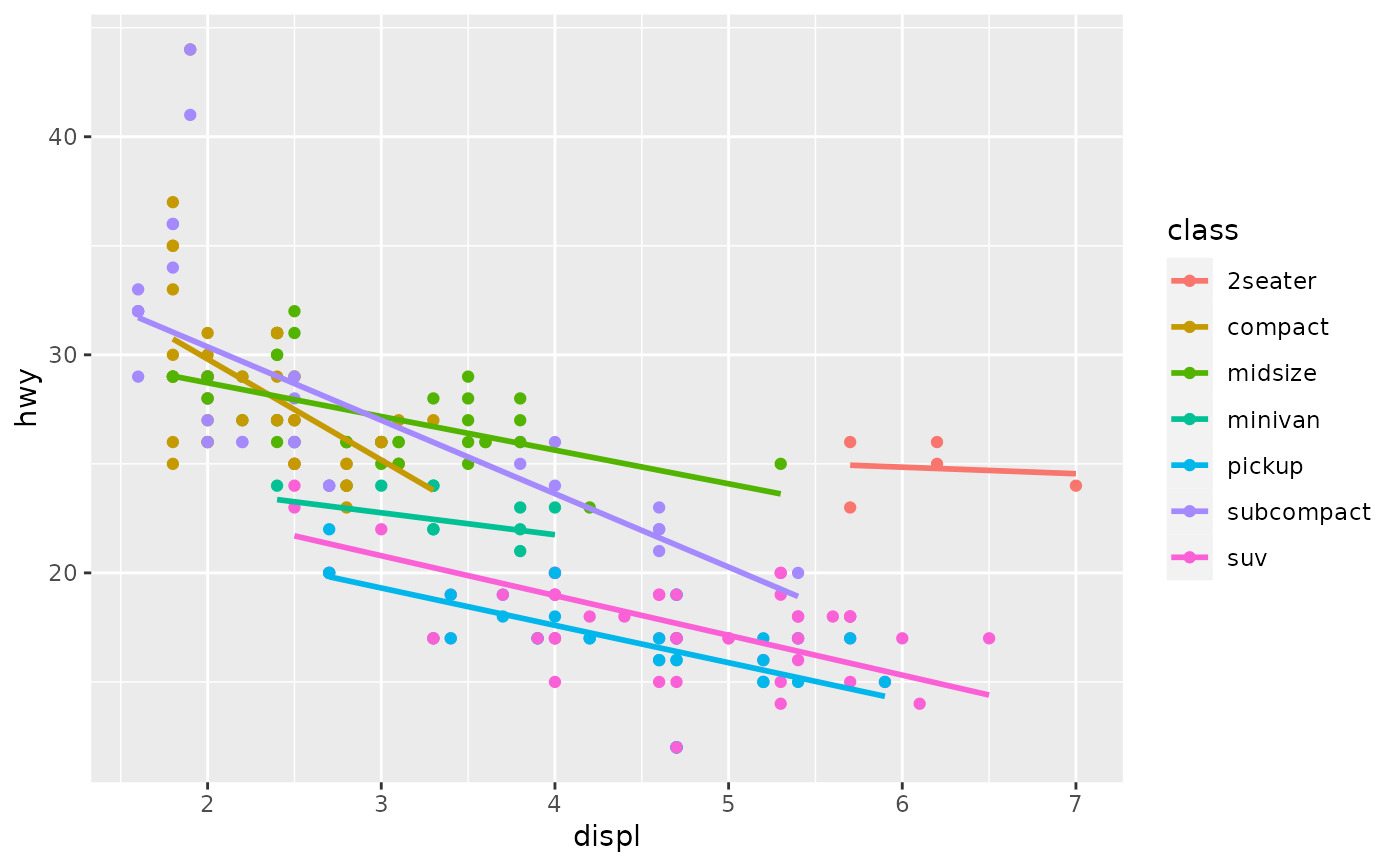
 # Smooths are automatically fit to each group (defined by categorical
# aesthetics or the group aesthetic) and for each facet.
ggplot(mpg, aes(displ, hwy, colour = class)) +
geom_point() +
geom_smooth(se = FALSE, method = lm)
#> `geom_smooth()` using formula = 'y ~ x'
# Smooths are automatically fit to each group (defined by categorical
# aesthetics or the group aesthetic) and for each facet.
ggplot(mpg, aes(displ, hwy, colour = class)) +
geom_point() +
geom_smooth(se = FALSE, method = lm)
#> `geom_smooth()` using formula = 'y ~ x'
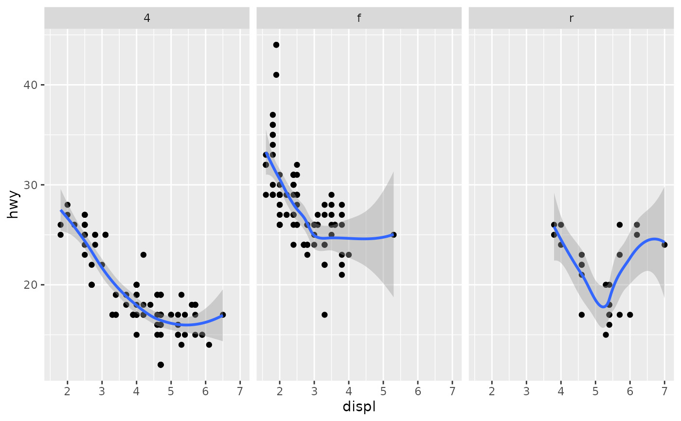
 ggplot(mpg, aes(displ, hwy)) +
geom_point() +
geom_smooth(span = 0.8) +
facet_wrap(~drv)
#> `geom_smooth()` using method = 'loess' and formula = 'y ~ x'
ggplot(mpg, aes(displ, hwy)) +
geom_point() +
geom_smooth(span = 0.8) +
facet_wrap(~drv)
#> `geom_smooth()` using method = 'loess' and formula = 'y ~ x'
 # \donttest{
binomial_smooth <- function(...) {
geom_smooth(method = "glm", method.args = list(family = "binomial"), ...)
}
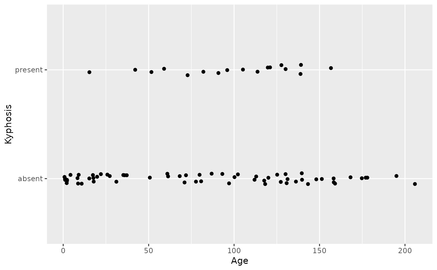
# To fit a logistic regression, you need to coerce the values to
# a numeric vector lying between 0 and 1.
ggplot(rpart::kyphosis, aes(Age, Kyphosis)) +
geom_jitter(height = 0.05) +
binomial_smooth()
#> `geom_smooth()` using formula = 'y ~ x'
#> Warning: Computation failed in `stat_smooth()`
#> Caused by error:
#> ! y values must be 0 <= y <= 1
# \donttest{
binomial_smooth <- function(...) {
geom_smooth(method = "glm", method.args = list(family = "binomial"), ...)
}
# To fit a logistic regression, you need to coerce the values to
# a numeric vector lying between 0 and 1.
ggplot(rpart::kyphosis, aes(Age, Kyphosis)) +
geom_jitter(height = 0.05) +
binomial_smooth()
#> `geom_smooth()` using formula = 'y ~ x'
#> Warning: Computation failed in `stat_smooth()`
#> Caused by error:
#> ! y values must be 0 <= y <= 1
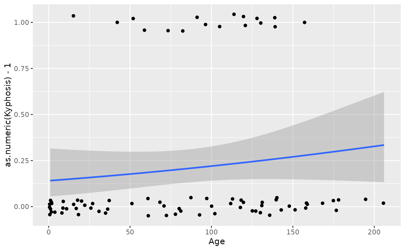
 ggplot(rpart::kyphosis, aes(Age, as.numeric(Kyphosis) - 1)) +
geom_jitter(height = 0.05) +
binomial_smooth()
#> `geom_smooth()` using formula = 'y ~ x'
ggplot(rpart::kyphosis, aes(Age, as.numeric(Kyphosis) - 1)) +
geom_jitter(height = 0.05) +
binomial_smooth()
#> `geom_smooth()` using formula = 'y ~ x'
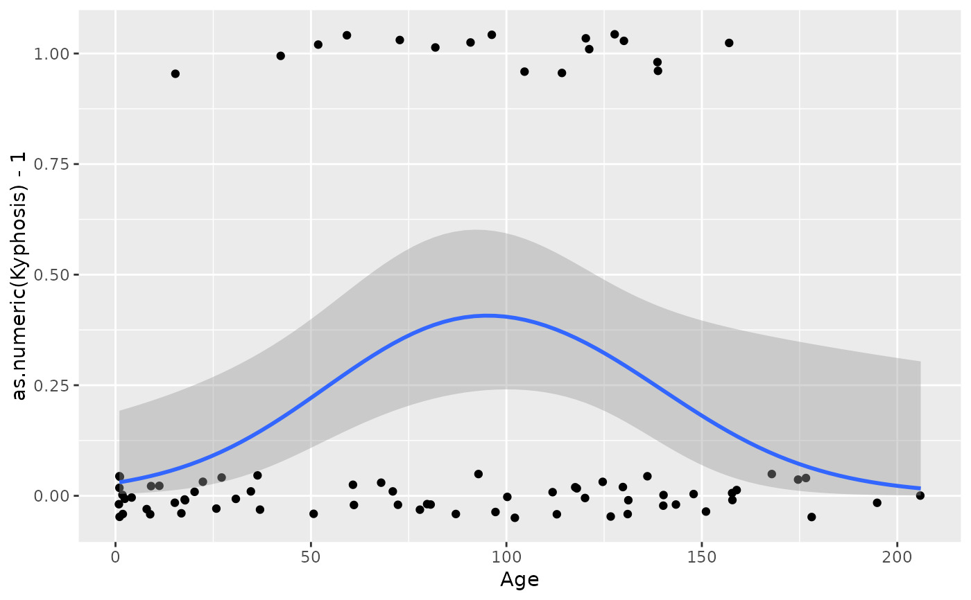
 ggplot(rpart::kyphosis, aes(Age, as.numeric(Kyphosis) - 1)) +
geom_jitter(height = 0.05) +
binomial_smooth(formula = y ~ splines::ns(x, 2))
ggplot(rpart::kyphosis, aes(Age, as.numeric(Kyphosis) - 1)) +
geom_jitter(height = 0.05) +
binomial_smooth(formula = y ~ splines::ns(x, 2))
 # But in this case, it's probably better to fit the model yourself
# so you can exercise more control and see whether or not it's a good model.
# }
# But in this case, it's probably better to fit the model yourself
# so you can exercise more control and see whether or not it's a good model.
# }
相關用法
- R ggplot2 geom_spoke 由位置、方向和距離參數化的線段
- R ggplot2 geom_segment 線段和曲線
- R ggplot2 geom_qq 分位數-分位數圖
- R ggplot2 geom_quantile 分位數回歸
- R ggplot2 geom_text 文本
- R ggplot2 geom_ribbon 函數區和麵積圖
- R ggplot2 geom_boxplot 盒須圖(Tukey 風格)
- R ggplot2 geom_hex 二維箱計數的六邊形熱圖
- R ggplot2 geom_bar 條形圖
- R ggplot2 geom_bin_2d 二維 bin 計數熱圖
- R ggplot2 geom_jitter 抖動點
- R ggplot2 geom_point 積分
- R ggplot2 geom_linerange 垂直間隔:線、橫線和誤差線
- R ggplot2 geom_blank 什麽也不畫
- R ggplot2 geom_path 連接觀察結果
- R ggplot2 geom_violin 小提琴情節
- R ggplot2 geom_dotplot 點圖
- R ggplot2 geom_errorbarh 水平誤差線
- R ggplot2 geom_function 將函數繪製為連續曲線
- R ggplot2 geom_polygon 多邊形
- R ggplot2 geom_histogram 直方圖和頻數多邊形
- R ggplot2 geom_tile 矩形
- R ggplot2 geom_density_2d 二維密度估計的等值線
- R ggplot2 geom_map 參考Map中的多邊形
- R ggplot2 geom_density 平滑密度估計
注:本文由純淨天空篩選整理自Hadley Wickham等大神的英文原創作品 Smoothed conditional means。非經特殊聲明,原始代碼版權歸原作者所有,本譯文未經允許或授權,請勿轉載或複製。