計算函數並將其繪製為連續曲線。這使得在現有繪圖上疊加函數變得很容易。使用沿 x 軸均勻分布的值的網格調用該函數,並用一條線繪製結果(默認情況下)。
用法
geom_function(
  mapping = NULL,
  data = NULL,
  stat = "function",
  position = "identity",
  ...,
  na.rm = FALSE,
  show.legend = NA,
  inherit.aes = TRUE
)

stat_function(
  mapping = NULL,
  data = NULL,
  geom = "function",
  position = "identity",
  ...,
  fun,
  xlim = NULL,
  n = 101,
  args = list(),
  na.rm = FALSE,
  show.legend = NA,
  inherit.aes = TRUE
)
參數
- mapping
-
由
aes()創建的一組美學映射。如果指定且inherit.aes = TRUE(默認),它將與繪圖頂層的默認映射組合。如果沒有繪圖映射,則必須提供mapping。 - data
-
被
stat_function()忽略,請勿使用。 - stat
-
用於該層數據的統計變換,可以作為
ggprotoGeom子類,也可以作為命名去掉stat_前綴的統計數據的字符串(例如"count"而不是"stat_count") - position
-
位置調整,可以是命名調整的字符串(例如
"jitter"使用position_jitter),也可以是調用位置調整函數的結果。如果需要更改調整設置,請使用後者。 - ...
-
其他參數傳遞給
layer()。這些通常是美學,用於將美學設置為固定值,例如colour = "red"或size = 3。它們也可能是配對的 geom/stat 的參數。 - na.rm
-
如果
FALSE,則默認缺失值將被刪除並帶有警告。如果TRUE,缺失值將被靜默刪除。 - show.legend
-
合乎邏輯的。該層是否應該包含在圖例中?
NA(默認值)包括是否映射了任何美學。FALSE從不包含,而TRUE始終包含。它也可以是一個命名的邏輯向量,以精細地選擇要顯示的美學。 - inherit.aes
-
如果
FALSE,則覆蓋默認美學,而不是與它們組合。這對於定義數據和美觀的輔助函數最有用,並且不應繼承默認繪圖規範的行為,例如borders()。 - geom
-
用於顯示數據的幾何對象,可以作為
ggprotoGeom子類,也可以作為命名去除geom_前綴的幾何對象的字符串(例如"point"而不是"geom_point") - fun
-
使用的函數。 1) 基本或 rlang 公式語法中的匿名函數(請參閱
rlang::as_function())或 2) 引用函數的帶引號或字符名稱;請參閱示例。必須矢量化。 - xlim
-
(可選)指定函數的範圍。
- n
-
沿 x 軸插值的點數。
- args
-
傳遞給
fun定義的函數的附加參數列表。
美學
geom_function() 理解以下美學(所需的美學以粗體顯示):
-
x -
y -
alpha -
colour -
group -
linetype -
linewidth
在 vignette("ggplot2-specs") 中了解有關設置這些美學的更多信息。
計算變量
這些是由層的 'stat' 部分計算的,可以使用 delayed evaluation 訪問。
-
after_stat(x)x沿網格的值。 -
after_stat(y)
函數的值在相應的位置評估x.
例子
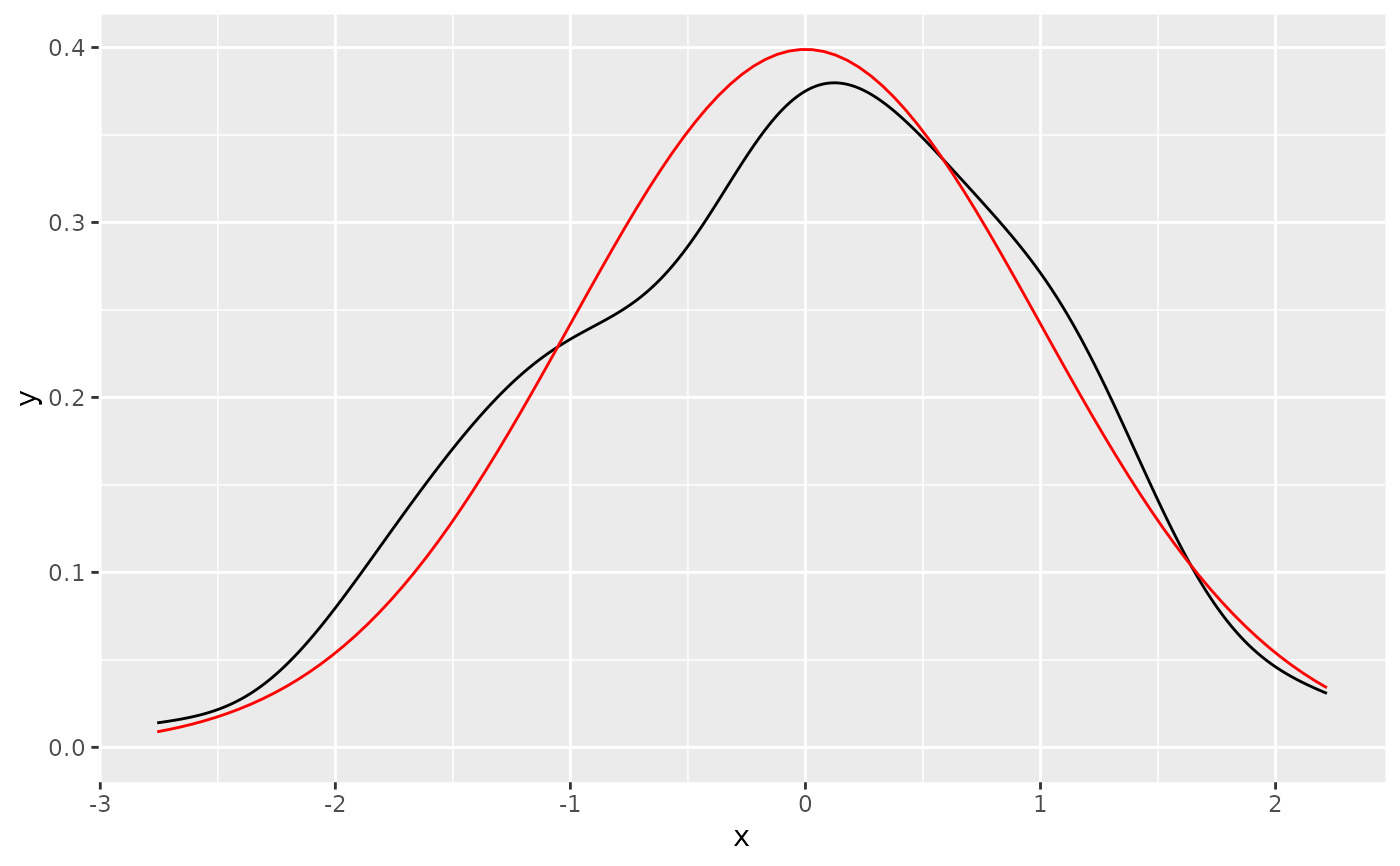
# geom_function() is useful for overlaying functions
set.seed(1492)
ggplot(data.frame(x = rnorm(100)), aes(x)) +
geom_density() +
geom_function(fun = dnorm, colour = "red")
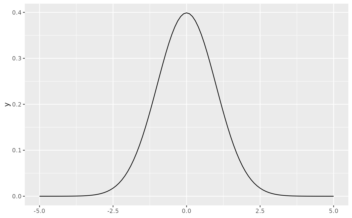
 # To plot functions without data, specify range of x-axis
base <-
ggplot() +
xlim(-5, 5)
base + geom_function(fun = dnorm)
# To plot functions without data, specify range of x-axis
base <-
ggplot() +
xlim(-5, 5)
base + geom_function(fun = dnorm)
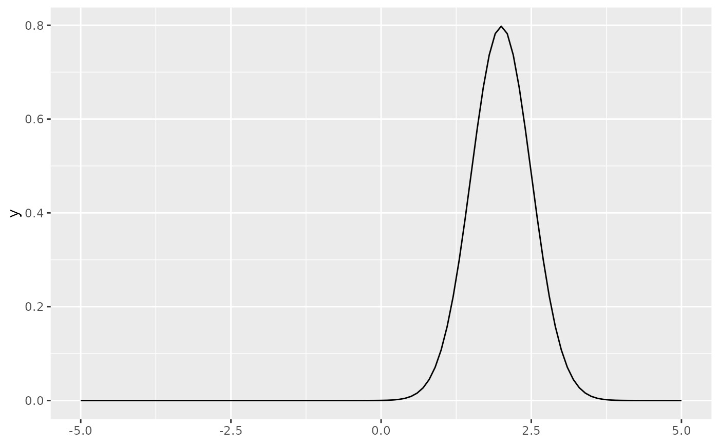
 base + geom_function(fun = dnorm, args = list(mean = 2, sd = .5))
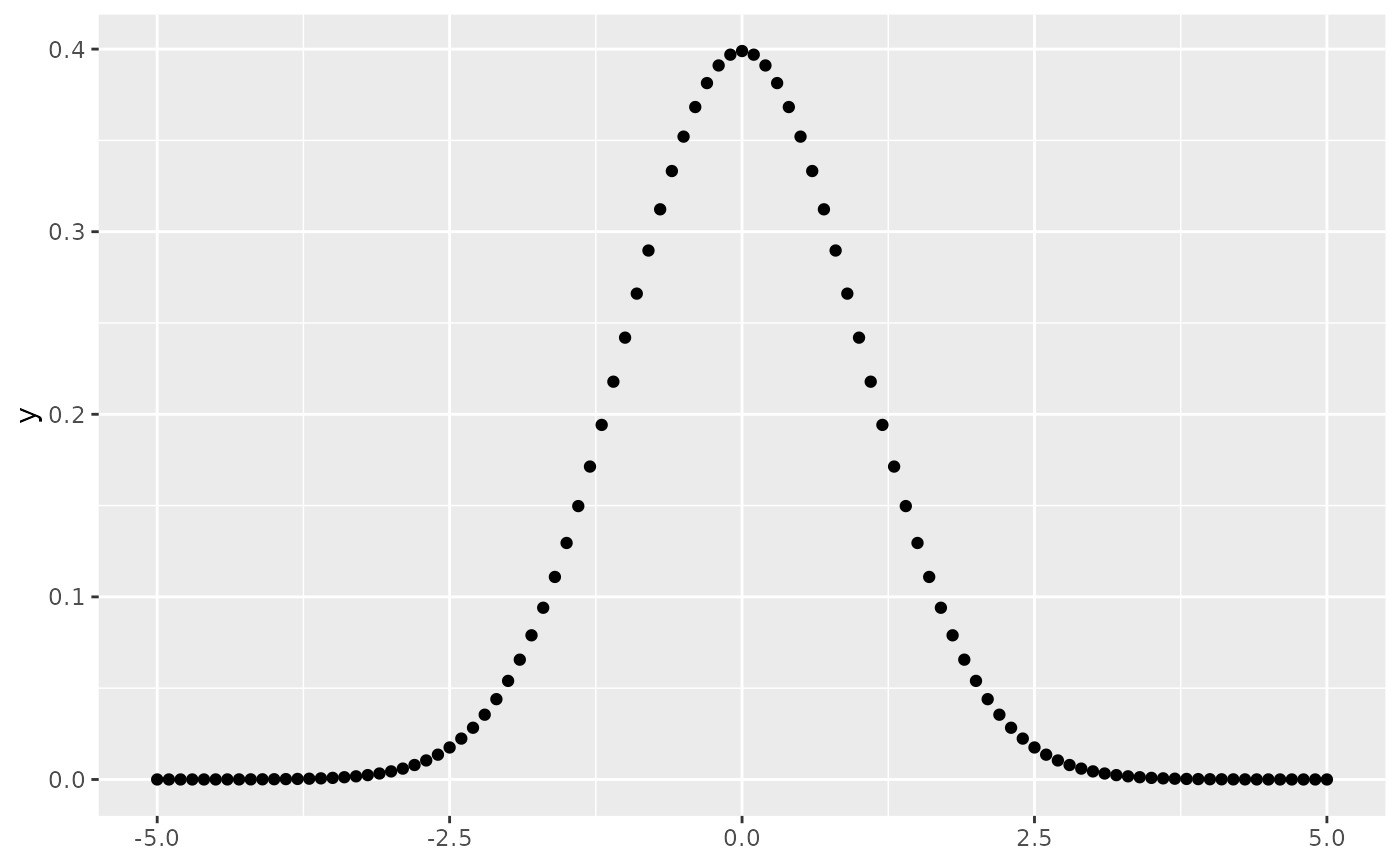
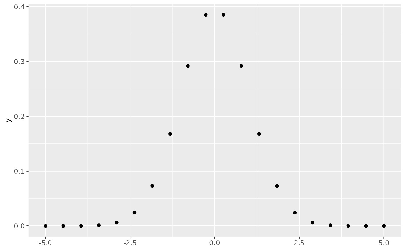
 # The underlying mechanics evaluate the function at discrete points
# and connect the points with lines
base + stat_function(fun = dnorm, geom = "point")
# The underlying mechanics evaluate the function at discrete points
# and connect the points with lines
base + stat_function(fun = dnorm, geom = "point")
 base + stat_function(fun = dnorm, geom = "point", n = 20)
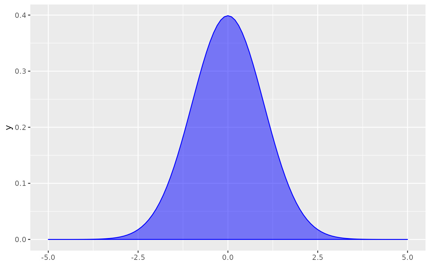
 base + stat_function(fun = dnorm, geom = "polygon", color = "blue", fill = "blue", alpha = 0.5)
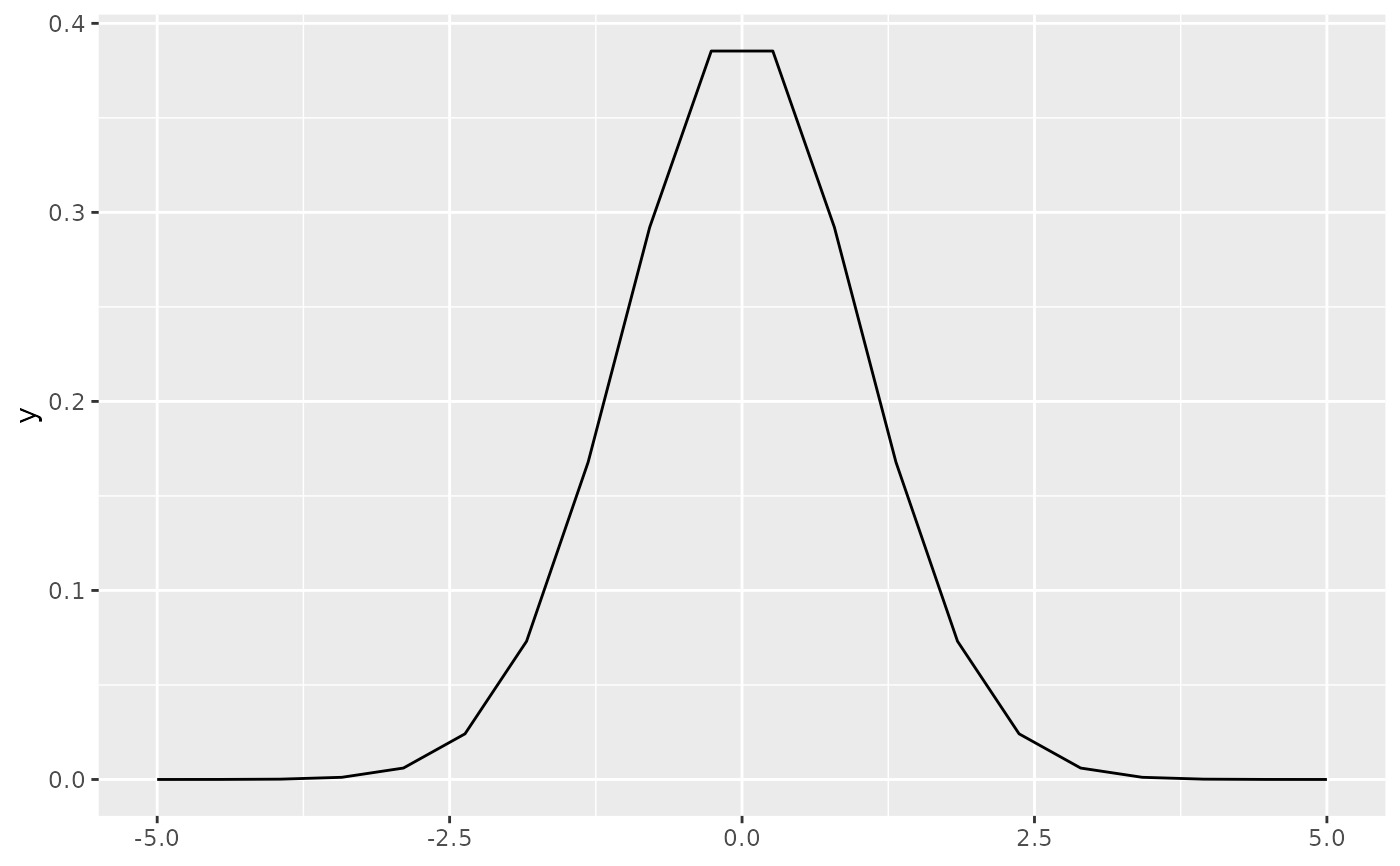
 base + geom_function(fun = dnorm, n = 20)
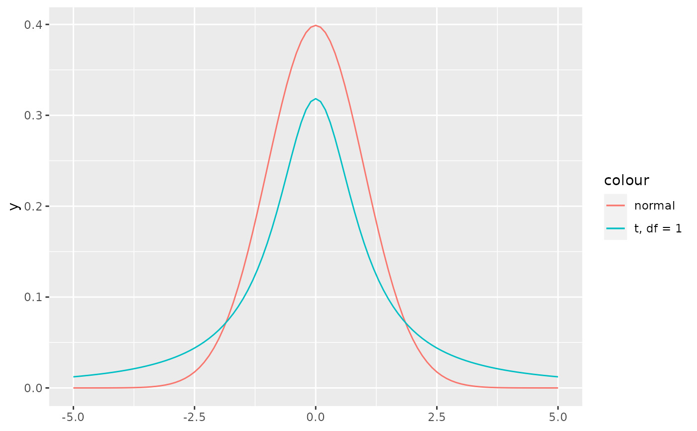
 # Two functions on the same plot
base +
geom_function(aes(colour = "normal"), fun = dnorm) +
geom_function(aes(colour = "t, df = 1"), fun = dt, args = list(df = 1))
# Two functions on the same plot
base +
geom_function(aes(colour = "normal"), fun = dnorm) +
geom_function(aes(colour = "t, df = 1"), fun = dt, args = list(df = 1))
 # Using a custom anonymous function
base + geom_function(fun = function(x) 0.5*exp(-abs(x)))
# Using a custom anonymous function
base + geom_function(fun = function(x) 0.5*exp(-abs(x)))
 base + geom_function(fun = ~ 0.5*exp(-abs(.x)))
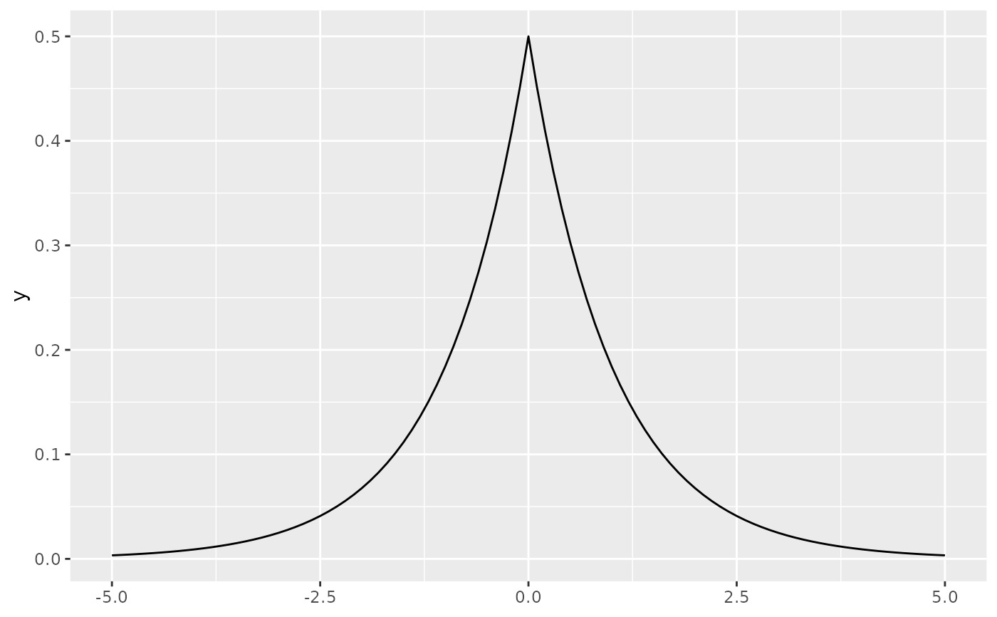 # Using a custom named function
f <- function(x) 0.5*exp(-abs(x))
base + geom_function(fun = f)
# Using a custom named function
f <- function(x) 0.5*exp(-abs(x))
base + geom_function(fun = f)
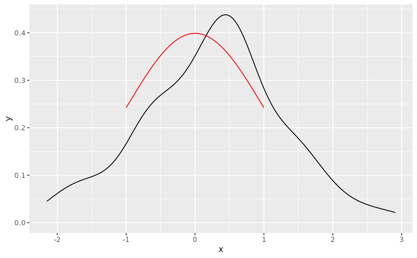
 # Using xlim to restrict the range of function
ggplot(data.frame(x = rnorm(100)), aes(x)) +
geom_density() +
geom_function(fun = dnorm, colour = "red", xlim=c(-1, 1))
# Using xlim to restrict the range of function
ggplot(data.frame(x = rnorm(100)), aes(x)) +
geom_density() +
geom_function(fun = dnorm, colour = "red", xlim=c(-1, 1))
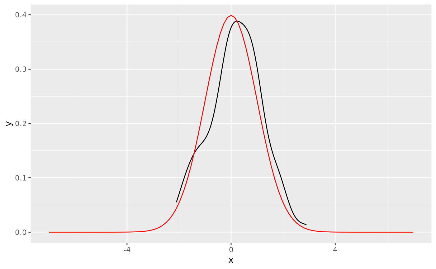
 # Using xlim to widen the range of function
ggplot(data.frame(x = rnorm(100)), aes(x)) +
geom_density() +
geom_function(fun = dnorm, colour = "red", xlim=c(-7, 7))
# Using xlim to widen the range of function
ggplot(data.frame(x = rnorm(100)), aes(x)) +
geom_density() +
geom_function(fun = dnorm, colour = "red", xlim=c(-7, 7))
相關用法
- R ggplot2 geom_qq 分位數-分位數圖
- R ggplot2 geom_spoke 由位置、方向和距離參數化的線段
- R ggplot2 geom_quantile 分位數回歸
- R ggplot2 geom_text 文本
- R ggplot2 geom_ribbon 函數區和麵積圖
- R ggplot2 geom_boxplot 盒須圖(Tukey 風格)
- R ggplot2 geom_hex 二維箱計數的六邊形熱圖
- R ggplot2 geom_bar 條形圖
- R ggplot2 geom_bin_2d 二維 bin 計數熱圖
- R ggplot2 geom_jitter 抖動點
- R ggplot2 geom_point 積分
- R ggplot2 geom_linerange 垂直間隔:線、橫線和誤差線
- R ggplot2 geom_blank 什麽也不畫
- R ggplot2 geom_path 連接觀察結果
- R ggplot2 geom_violin 小提琴情節
- R ggplot2 geom_dotplot 點圖
- R ggplot2 geom_errorbarh 水平誤差線
- R ggplot2 geom_polygon 多邊形
- R ggplot2 geom_histogram 直方圖和頻數多邊形
- R ggplot2 geom_tile 矩形
- R ggplot2 geom_segment 線段和曲線
- R ggplot2 geom_density_2d 二維密度估計的等值線
- R ggplot2 geom_map 參考Map中的多邊形
- R ggplot2 geom_density 平滑密度估計
- R ggplot2 geom_abline 參考線:水平、垂直和對角線
注:本文由純淨天空篩選整理自Hadley Wickham等大神的英文原創作品 Draw a function as a continuous curve。非經特殊聲明,原始代碼版權歸原作者所有,本譯文未經允許或授權,請勿轉載或複製。