计算函数并将其绘制为连续曲线。这使得在现有绘图上叠加函数变得很容易。使用沿 x 轴均匀分布的值的网格调用该函数,并用一条线绘制结果(默认情况下)。
用法
geom_function(
  mapping = NULL,
  data = NULL,
  stat = "function",
  position = "identity",
  ...,
  na.rm = FALSE,
  show.legend = NA,
  inherit.aes = TRUE
)

stat_function(
  mapping = NULL,
  data = NULL,
  geom = "function",
  position = "identity",
  ...,
  fun,
  xlim = NULL,
  n = 101,
  args = list(),
  na.rm = FALSE,
  show.legend = NA,
  inherit.aes = TRUE
)
参数
- mapping
-
由
aes()创建的一组美学映射。如果指定且inherit.aes = TRUE(默认),它将与绘图顶层的默认映射组合。如果没有绘图映射,则必须提供mapping。 - data
-
被
stat_function()忽略,请勿使用。 - stat
-
用于该层数据的统计变换,可以作为
ggprotoGeom子类,也可以作为命名去掉stat_前缀的统计数据的字符串(例如"count"而不是"stat_count") - position
-
位置调整,可以是命名调整的字符串(例如
"jitter"使用position_jitter),也可以是调用位置调整函数的结果。如果需要更改调整设置,请使用后者。 - ...
-
其他参数传递给
layer()。这些通常是美学,用于将美学设置为固定值,例如colour = "red"或size = 3。它们也可能是配对的 geom/stat 的参数。 - na.rm
-
如果
FALSE,则默认缺失值将被删除并带有警告。如果TRUE,缺失值将被静默删除。 - show.legend
-
合乎逻辑的。该层是否应该包含在图例中?
NA(默认值)包括是否映射了任何美学。FALSE从不包含,而TRUE始终包含。它也可以是一个命名的逻辑向量,以精细地选择要显示的美学。 - inherit.aes
-
如果
FALSE,则覆盖默认美学,而不是与它们组合。这对于定义数据和美观的辅助函数最有用,并且不应继承默认绘图规范的行为,例如borders()。 - geom
-
用于显示数据的几何对象,可以作为
ggprotoGeom子类,也可以作为命名去除geom_前缀的几何对象的字符串(例如"point"而不是"geom_point") - fun
-
使用的函数。 1) 基本或 rlang 公式语法中的匿名函数(请参阅
rlang::as_function())或 2) 引用函数的带引号或字符名称;请参阅示例。必须矢量化。 - xlim
-
(可选)指定函数的范围。
- n
-
沿 x 轴插值的点数。
- args
-
传递给
fun定义的函数的附加参数列表。
美学
geom_function() 理解以下美学(所需的美学以粗体显示):
-
x -
y -
alpha -
colour -
group -
linetype -
linewidth
在 vignette("ggplot2-specs") 中了解有关设置这些美学的更多信息。
计算变量
这些是由层的 'stat' 部分计算的,可以使用 delayed evaluation 访问。
-
after_stat(x)x沿网格的值。 -
after_stat(y)
函数的值在相应的位置评估x.
例子
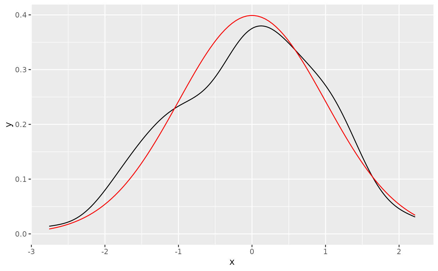
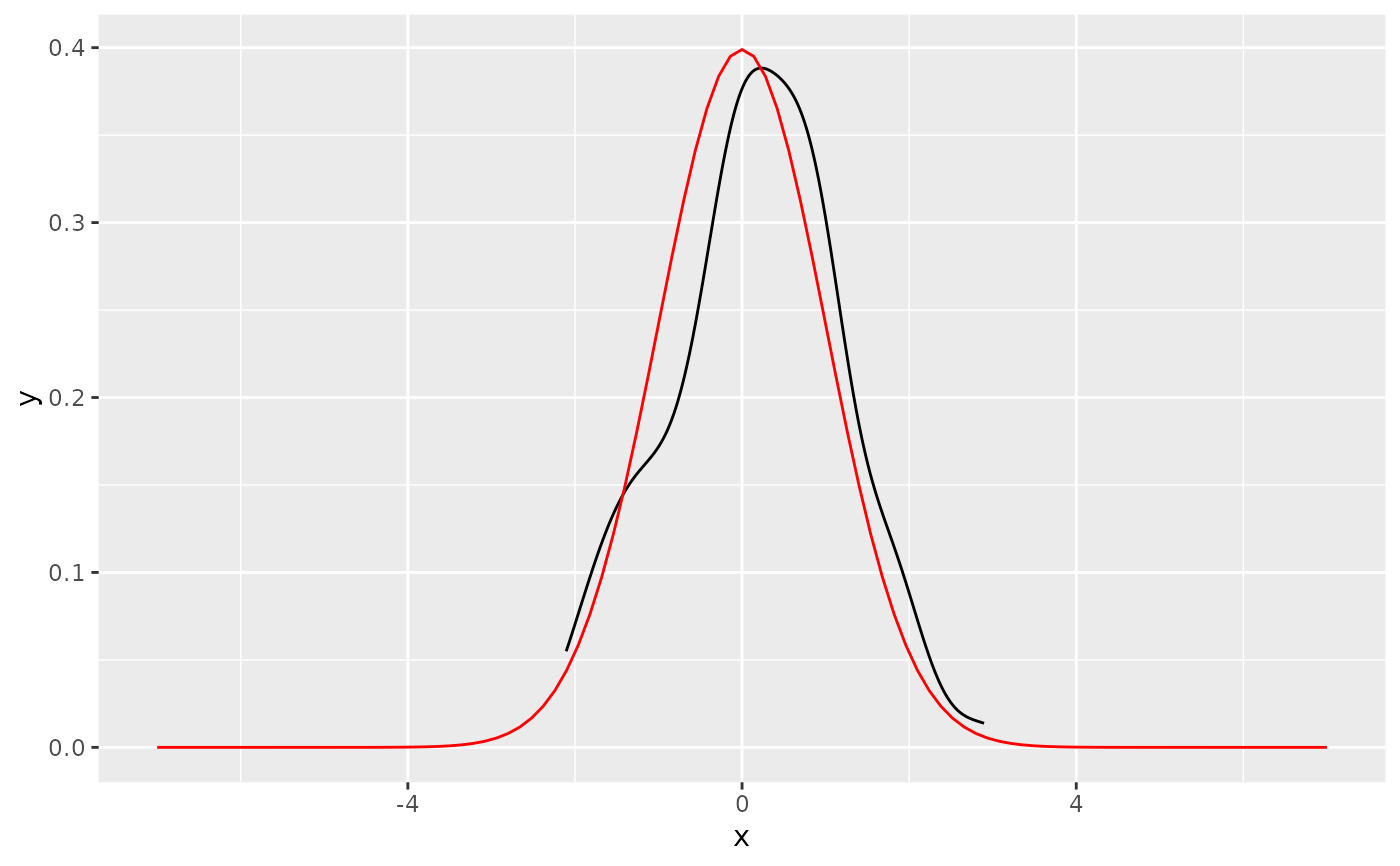
# geom_function() is useful for overlaying functions
set.seed(1492)
ggplot(data.frame(x = rnorm(100)), aes(x)) +
geom_density() +
geom_function(fun = dnorm, colour = "red")
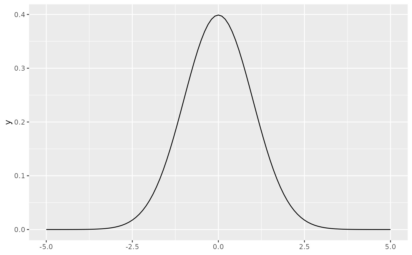
 # To plot functions without data, specify range of x-axis
base <-
ggplot() +
xlim(-5, 5)
base + geom_function(fun = dnorm)
# To plot functions without data, specify range of x-axis
base <-
ggplot() +
xlim(-5, 5)
base + geom_function(fun = dnorm)
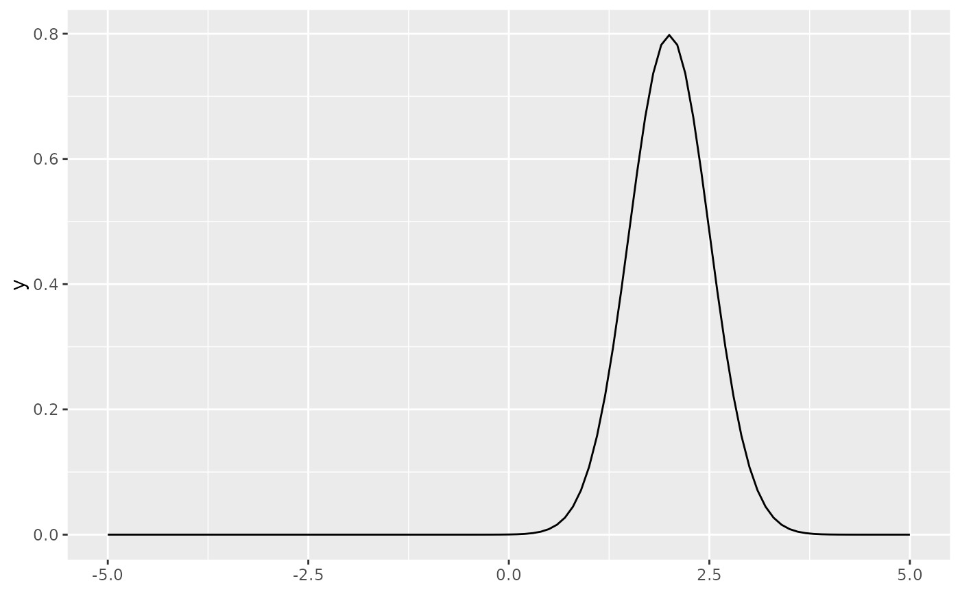
 base + geom_function(fun = dnorm, args = list(mean = 2, sd = .5))
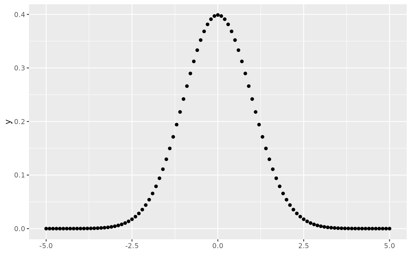
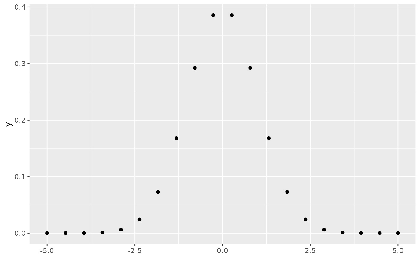
 # The underlying mechanics evaluate the function at discrete points
# and connect the points with lines
base + stat_function(fun = dnorm, geom = "point")
# The underlying mechanics evaluate the function at discrete points
# and connect the points with lines
base + stat_function(fun = dnorm, geom = "point")
 base + stat_function(fun = dnorm, geom = "point", n = 20)
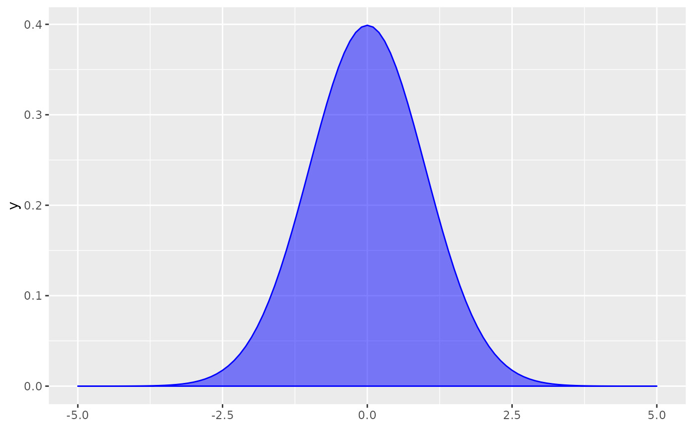
 base + stat_function(fun = dnorm, geom = "polygon", color = "blue", fill = "blue", alpha = 0.5)
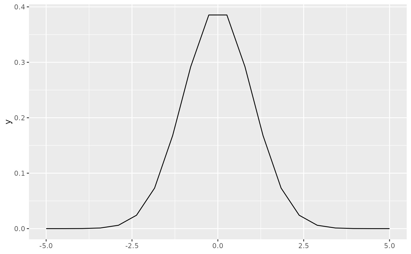
 base + geom_function(fun = dnorm, n = 20)
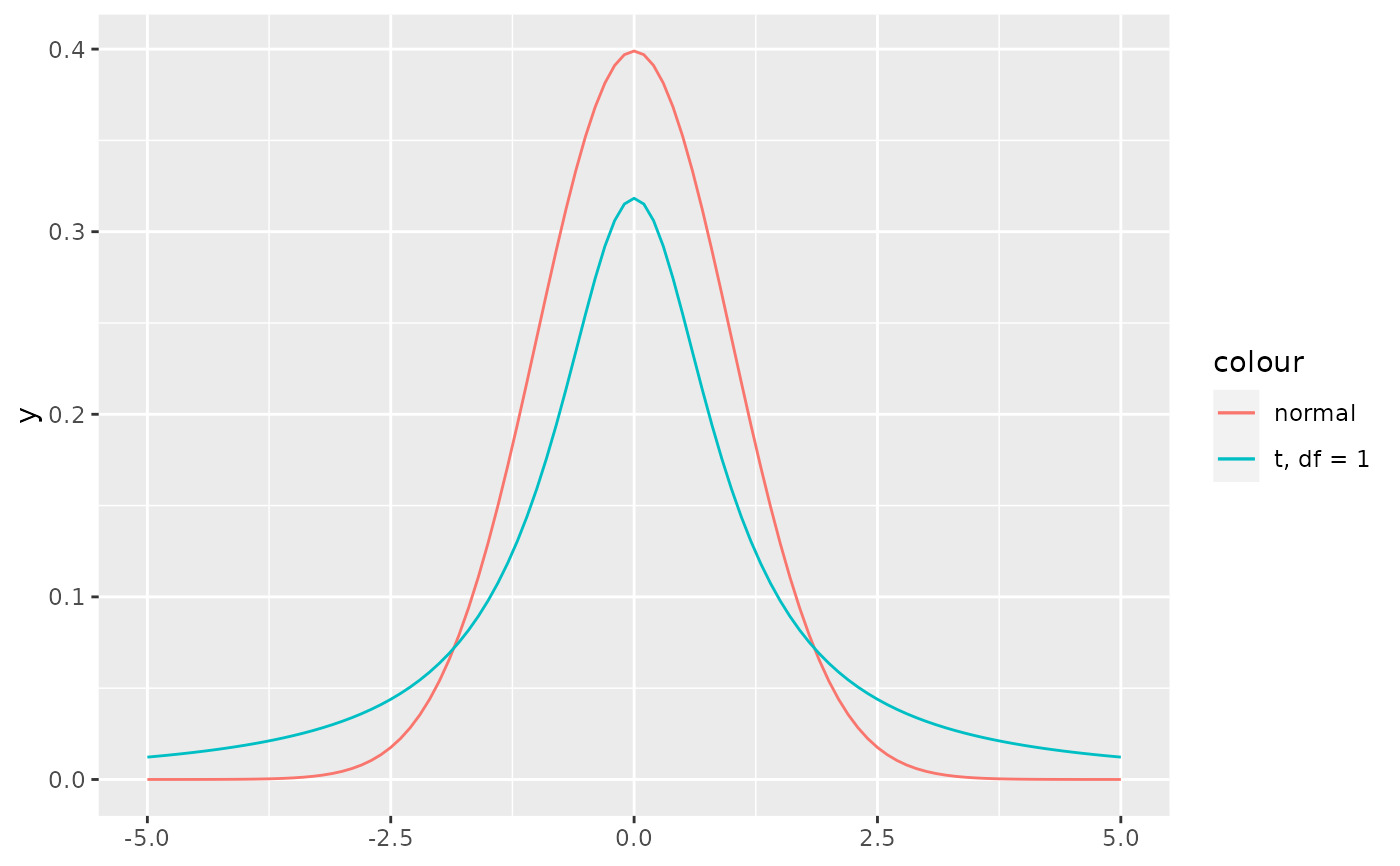
 # Two functions on the same plot
base +
geom_function(aes(colour = "normal"), fun = dnorm) +
geom_function(aes(colour = "t, df = 1"), fun = dt, args = list(df = 1))
# Two functions on the same plot
base +
geom_function(aes(colour = "normal"), fun = dnorm) +
geom_function(aes(colour = "t, df = 1"), fun = dt, args = list(df = 1))
 # Using a custom anonymous function
base + geom_function(fun = function(x) 0.5*exp(-abs(x)))
# Using a custom anonymous function
base + geom_function(fun = function(x) 0.5*exp(-abs(x)))
 base + geom_function(fun = ~ 0.5*exp(-abs(.x)))
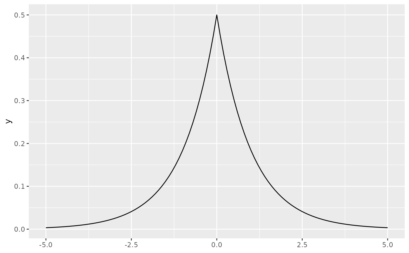 # Using a custom named function
f <- function(x) 0.5*exp(-abs(x))
base + geom_function(fun = f)
# Using a custom named function
f <- function(x) 0.5*exp(-abs(x))
base + geom_function(fun = f)
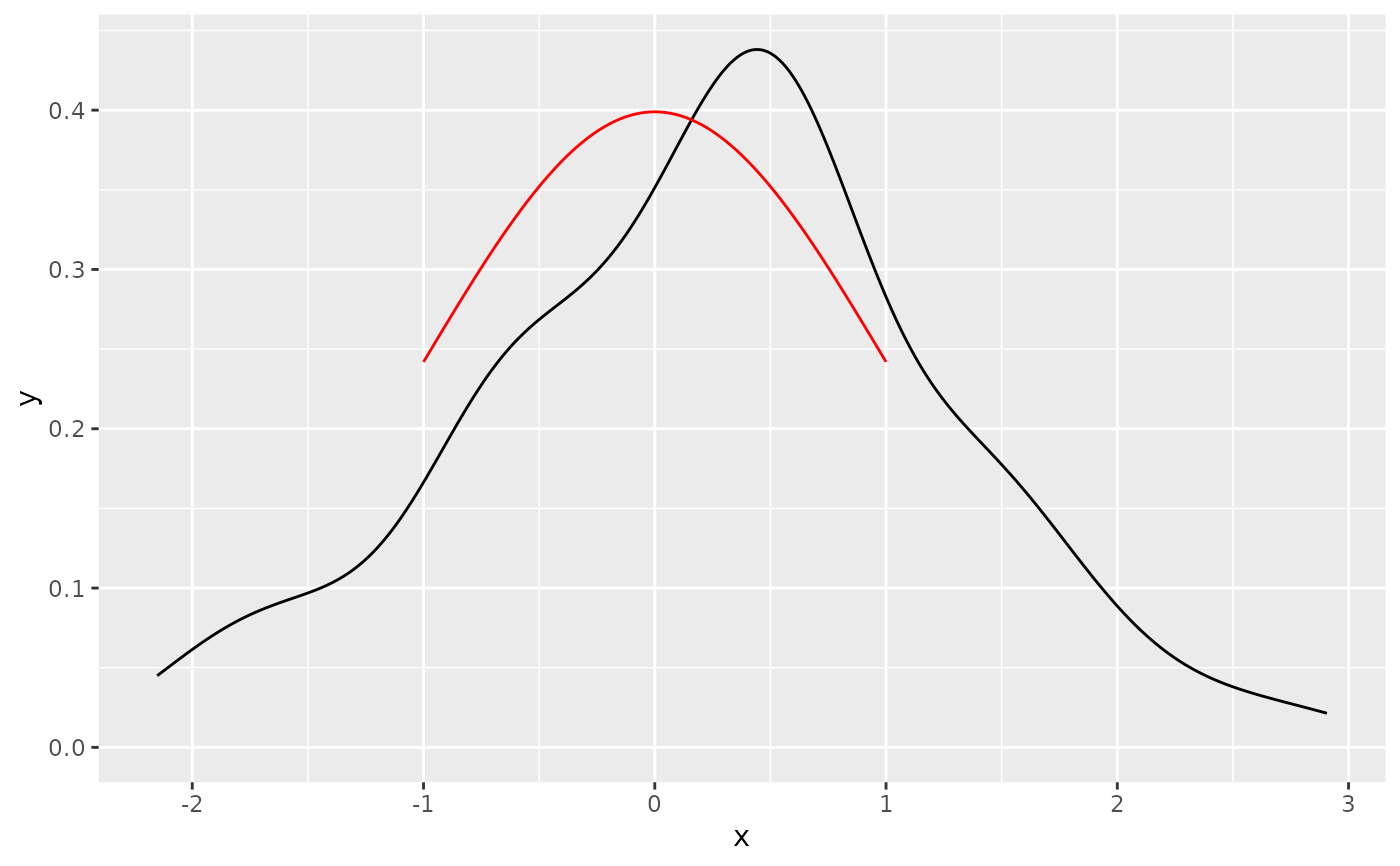
 # Using xlim to restrict the range of function
ggplot(data.frame(x = rnorm(100)), aes(x)) +
geom_density() +
geom_function(fun = dnorm, colour = "red", xlim=c(-1, 1))
# Using xlim to restrict the range of function
ggplot(data.frame(x = rnorm(100)), aes(x)) +
geom_density() +
geom_function(fun = dnorm, colour = "red", xlim=c(-1, 1))
 # Using xlim to widen the range of function
ggplot(data.frame(x = rnorm(100)), aes(x)) +
geom_density() +
geom_function(fun = dnorm, colour = "red", xlim=c(-7, 7))
# Using xlim to widen the range of function
ggplot(data.frame(x = rnorm(100)), aes(x)) +
geom_density() +
geom_function(fun = dnorm, colour = "red", xlim=c(-7, 7))
相关用法
- R ggplot2 geom_qq 分位数-分位数图
- R ggplot2 geom_spoke 由位置、方向和距离参数化的线段
- R ggplot2 geom_quantile 分位数回归
- R ggplot2 geom_text 文本
- R ggplot2 geom_ribbon 函数区和面积图
- R ggplot2 geom_boxplot 盒须图(Tukey 风格)
- R ggplot2 geom_hex 二维箱计数的六边形热图
- R ggplot2 geom_bar 条形图
- R ggplot2 geom_bin_2d 二维 bin 计数热图
- R ggplot2 geom_jitter 抖动点
- R ggplot2 geom_point 积分
- R ggplot2 geom_linerange 垂直间隔:线、横线和误差线
- R ggplot2 geom_blank 什么也不画
- R ggplot2 geom_path 连接观察结果
- R ggplot2 geom_violin 小提琴情节
- R ggplot2 geom_dotplot 点图
- R ggplot2 geom_errorbarh 水平误差线
- R ggplot2 geom_polygon 多边形
- R ggplot2 geom_histogram 直方图和频数多边形
- R ggplot2 geom_tile 矩形
- R ggplot2 geom_segment 线段和曲线
- R ggplot2 geom_density_2d 二维密度估计的等值线
- R ggplot2 geom_map 参考Map中的多边形
- R ggplot2 geom_density 平滑密度估计
- R ggplot2 geom_abline 参考线:水平、垂直和对角线
注:本文由纯净天空筛选整理自Hadley Wickham等大神的英文原创作品 Draw a function as a continuous curve。非经特殊声明,原始代码版权归原作者所有,本译文未经允许或授权,请勿转载或复制。