R ggplot2 geom_map 参考Map中的多边形

将多边形显示为Map。这意味着注释，因此它不会影响位置比例。请注意，此函数早于 geom_sf() 框架，并且不适用于 sf 几何列作为输入。但是，它可以与 geom_sf() 层和/或 coord_sf() 结合使用(请参阅示例)。

用法

geom_map(
  mapping = NULL,
  data = NULL,
  stat = "identity",
  ...,
  map,
  na.rm = FALSE,
  show.legend = NA,
  inherit.aes = TRUE
)

参数

mapping

由 aes() 创建的一组美学映射。如果指定且inherit.aes = TRUE(默认)，它将与绘图顶层的默认映射组合。如果没有绘图映射，则必须提供mapping。

data

该层要显示的数据。有以下三种选择：

如果默认为 NULL ，则数据继承自 ggplot() 调用中指定的绘图数据。

data.frame 或其他对象将覆盖绘图数据。所有对象都将被强化以生成 DataFrame 。请参阅fortify() 将为其创建变量。

将使用单个参数(绘图数据)调用function。返回值必须是 data.frame ，并将用作图层数据。可以从 formula 创建 function (例如 ~ head(.x, 10) )。

stat

用于该层数据的统计变换，可以作为 ggproto Geom 子类，也可以作为命名去掉 stat_ 前缀的统计数据的字符串(例如 "count" 而不是 "stat_count" )

...

其他参数传递给 layer() 。这些通常是美学，用于将美学设置为固定值，例如 colour = "red" 或 size = 3 。它们也可能是配对的 geom/stat 的参数。

map

包含Map坐标的 DataFrame 。这通常是在空间对象上使用 fortify() 创建的。它必须包含列 x 或 long 、 y 或 lat 以及 region 或 id 。

na.rm

如果 FALSE ，则默认缺失值将被删除并带有警告。如果 TRUE ，缺失值将被静默删除。

show.legend

合乎逻辑的。该层是否应该包含在图例中？ NA(默认值)包括是否映射了任何美学。 FALSE 从不包含，而 TRUE 始终包含。它也可以是一个命名的逻辑向量，以精细地选择要显示的美学。

inherit.aes

如果 FALSE ，则覆盖默认美学，而不是与它们组合。这对于定义数据和美观的辅助函数最有用，并且不应继承默认绘图规范的行为，例如borders() 。

美学

geom_map() 理解以下美学(所需的美学以粗体显示)：

map_id
alpha
colour
fill
group
linetype
linewidth
subgroup

在 vignette("ggplot2-specs") 中了解有关设置这些美学的更多信息。

例子

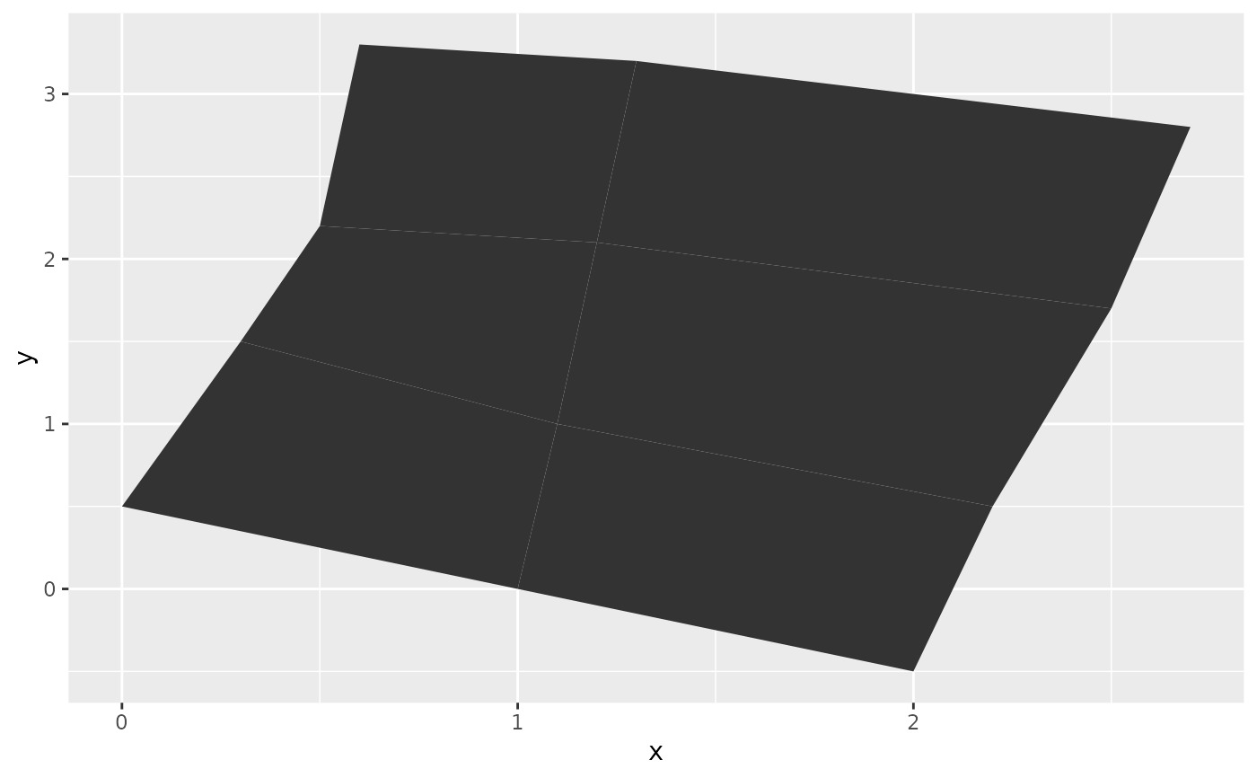
# First, a made-up example containing a few polygons, to explain
# how `geom_map()` works. It requires two data frames:
# One contains the coordinates of each polygon (`positions`), and is
# provided via the `map` argument. The other contains the
# other the values associated with each polygon (`values`).  An id
# variable links the two together.

ids <- factor(c("1.1", "2.1", "1.2", "2.2", "1.3", "2.3"))

values <- data.frame(
  id = ids,
  value = c(3, 3.1, 3.1, 3.2, 3.15, 3.5)
)

positions <- data.frame(
  id = rep(ids, each = 4),
  x = c(2, 1, 1.1, 2.2, 1, 0, 0.3, 1.1, 2.2, 1.1, 1.2, 2.5, 1.1, 0.3,
  0.5, 1.2, 2.5, 1.2, 1.3, 2.7, 1.2, 0.5, 0.6, 1.3),
  y = c(-0.5, 0, 1, 0.5, 0, 0.5, 1.5, 1, 0.5, 1, 2.1, 1.7, 1, 1.5,
  2.2, 2.1, 1.7, 2.1, 3.2, 2.8, 2.1, 2.2, 3.3, 3.2)
)

ggplot(values) +
  geom_map(aes(map_id = id), map = positions) +
  expand_limits(positions)

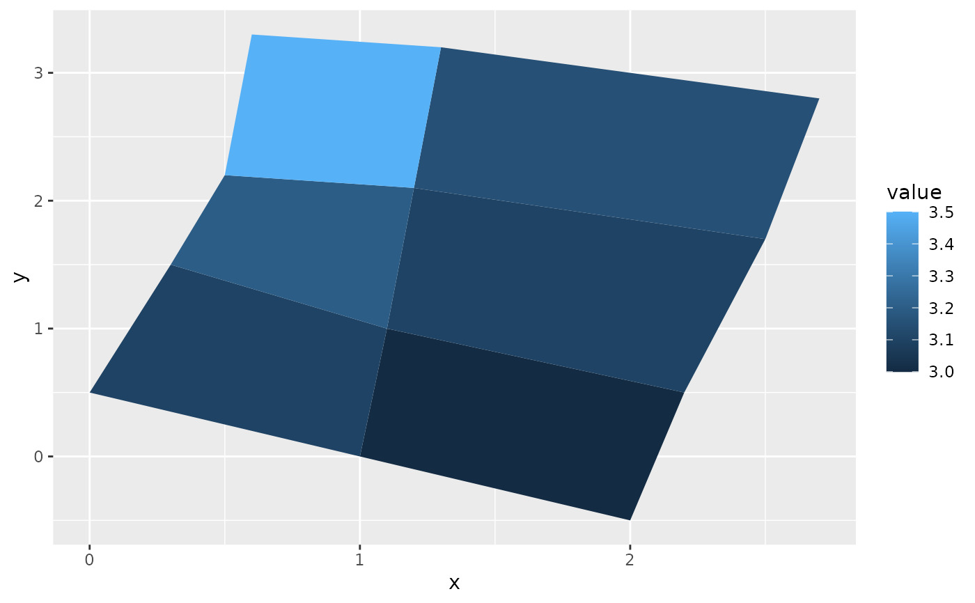
ggplot(values, aes(fill = value)) +
  geom_map(aes(map_id = id), map = positions) +
  expand_limits(positions)

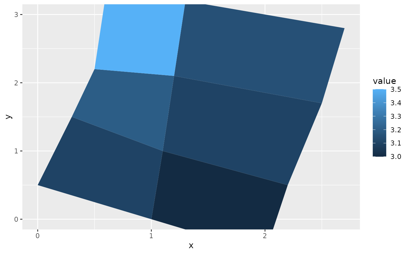
ggplot(values, aes(fill = value)) +
  geom_map(aes(map_id = id), map = positions) +
  expand_limits(positions) + ylim(0, 3)


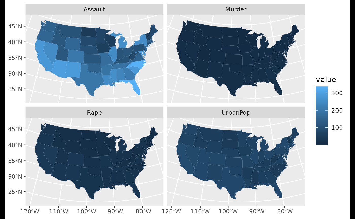
# Now some examples with real maps
if (require(maps)) {

  crimes <- data.frame(state = tolower(rownames(USArrests)), USArrests)

  # Equivalent to crimes %>% tidyr::pivot_longer(Murder:Rape)
  vars <- lapply(names(crimes)[-1], function(j) {
    data.frame(state = crimes$state, variable = j, value = crimes[[j]])
  })
  crimes_long <- do.call("rbind", vars)

  states_map <- map_data("state")

  # without geospatial coordinate system, the resulting plot
  # looks weird
  ggplot(crimes, aes(map_id = state)) +
    geom_map(aes(fill = Murder), map = states_map) +
    expand_limits(x = states_map$long, y = states_map$lat)

  # in combination with `coord_sf()` we get an appropriate result
  ggplot(crimes, aes(map_id = state)) +
    geom_map(aes(fill = Murder), map = states_map) +
    # crs = 5070 is a Conus Albers projection for North America,
    #   see: https://epsg.io/5070
    # default_crs = 4326 tells coord_sf() that the input map data
    #   are in longitude-latitude format
    coord_sf(
      crs = 5070, default_crs = 4326,
      xlim = c(-125, -70), ylim = c(25, 52)
    )

 ggplot(crimes_long, aes(map_id = state)) +
   geom_map(aes(fill = value), map = states_map) +
   coord_sf(
     crs = 5070, default_crs = 4326,
     xlim = c(-125, -70), ylim = c(25, 52)
   ) +
   facet_wrap(~variable)
}

源代码：R/geom-map.R

相关用法

注：本文由纯净天空筛选整理自Hadley Wickham等大神的英文原创作品 Polygons from a reference map。非经特殊声明，原始代码版权归原作者所有，本译文未经允许或授权，请勿转载或复制。