geom_path() 按照观测值在数据中出现的顺序连接它们。 geom_line() 按照 x 轴上的变量顺序将它们连接起来。 geom_step() 创建一个阶梯图,准确突出显示更改发生的时间。 group 美学决定了哪些案例连接在一起。
用法
geom_path(
  mapping = NULL,
  data = NULL,
  stat = "identity",
  position = "identity",
  ...,
  lineend = "butt",
  linejoin = "round",
  linemitre = 10,
  arrow = NULL,
  na.rm = FALSE,
  show.legend = NA,
  inherit.aes = TRUE
)

geom_line(
  mapping = NULL,
  data = NULL,
  stat = "identity",
  position = "identity",
  na.rm = FALSE,
  orientation = NA,
  show.legend = NA,
  inherit.aes = TRUE,
  ...
)

geom_step(
  mapping = NULL,
  data = NULL,
  stat = "identity",
  position = "identity",
  direction = "hv",
  na.rm = FALSE,
  show.legend = NA,
  inherit.aes = TRUE,
  ...
)
参数
- mapping
-
由
aes()创建的一组美学映射。如果指定且inherit.aes = TRUE(默认),它将与绘图顶层的默认映射组合。如果没有绘图映射,则必须提供mapping。 - data
-
该层要显示的数据。有以下三种选择:
如果默认为
NULL,则数据继承自ggplot()调用中指定的绘图数据。data.frame或其他对象将覆盖绘图数据。所有对象都将被强化以生成 DataFrame 。请参阅fortify()将为其创建变量。将使用单个参数(绘图数据)调用
function。返回值必须是data.frame,并将用作图层数据。可以从formula创建function(例如~ head(.x, 10))。 - stat
-
用于该层数据的统计变换,可以作为
ggprotoGeom子类,也可以作为命名去掉stat_前缀的统计数据的字符串(例如"count"而不是"stat_count") - position
-
位置调整,可以是命名调整的字符串(例如
"jitter"使用position_jitter),也可以是调用位置调整函数的结果。如果需要更改调整设置,请使用后者。 - ...
-
其他参数传递给
layer()。这些通常是美学,用于将美学设置为固定值,例如colour = "red"或size = 3。它们也可能是配对的 geom/stat 的参数。 - lineend
-
线端样式(圆形、对接、方形)。
- linejoin
-
线连接样式(圆形、斜接、斜角)。
- linemitre
-
线斜接限制(数量大于 1)。
- arrow
-
箭头规范,由
grid::arrow()创建。 - na.rm
-
如果
FALSE,则默认缺失值将被删除并带有警告。如果TRUE,缺失值将被静默删除。 - show.legend
-
合乎逻辑的。该层是否应该包含在图例中?
NA(默认值)包括是否映射了任何美学。FALSE从不包含,而TRUE始终包含。它也可以是一个命名的逻辑向量,以精细地选择要显示的美学。 - inherit.aes
-
如果
FALSE,则覆盖默认美学,而不是与它们组合。这对于定义数据和美观的辅助函数最有用,并且不应继承默认绘图规范的行为,例如borders()。 - orientation
-
层的方向。默认值 (
NA) 自动根据美学映射确定方向。万一失败,可以通过将orientation设置为"x"或"y"来显式给出。有关更多详细信息,请参阅方向部分。 - direction
-
楼梯方向:'vh'表示垂直然后水平,'hv'表示水平然后垂直,或'mid'表示相邻x-values之间的台阶half-way。
细节
另一种参数化是 geom_segment() ,其中每行对应一个提供开始和结束坐标的案例。
方向
该几何体以不同的方式对待每个轴,因此可以有两个方向。通常,方向很容易从给定映射和使用的位置比例类型的组合中推断出来。因此,ggplot2 默认情况下会尝试猜测图层应具有哪个方向。在极少数情况下,方向不明确,猜测可能会失败。在这种情况下,可以直接使用 orientation 参数指定方向,该参数可以是 "x" 或 "y" 。该值给出了几何图形应沿着的轴,"x" 是您期望的几何图形的默认方向。
美学
geom_path() 理解以下美学(所需的美学以粗体显示):
-
x -
y -
alpha -
colour -
group -
linetype -
linewidth
在 vignette("ggplot2-specs") 中了解有关设置这些美学的更多信息。
缺失值处理
geom_path() 、 geom_line() 和 geom_step() 处理 NA 如下:
-
如果
NA出现在一行的中间,则会中断该行。无论na.rm是TRUE还是FALSE,都不会显示警告。 -
如果
NA出现在行的开头或结尾,并且na.rm是FALSE(默认),则删除NA并发出警告。 -
如果
NA出现在行的开头或结尾,并且na.rm是TRUE,则NA将被静默删除,而不发出警告。
也可以看看
geom_polygon():填充路径(多边形); geom_segment():线段
例子
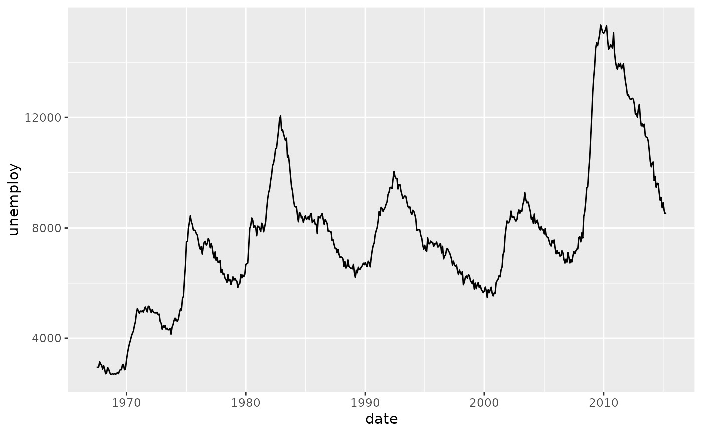
# geom_line() is suitable for time series
ggplot(economics, aes(date, unemploy)) + geom_line()
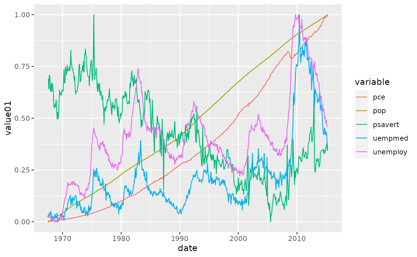
 ggplot(economics_long, aes(date, value01, colour = variable)) +
geom_line()
ggplot(economics_long, aes(date, value01, colour = variable)) +
geom_line()
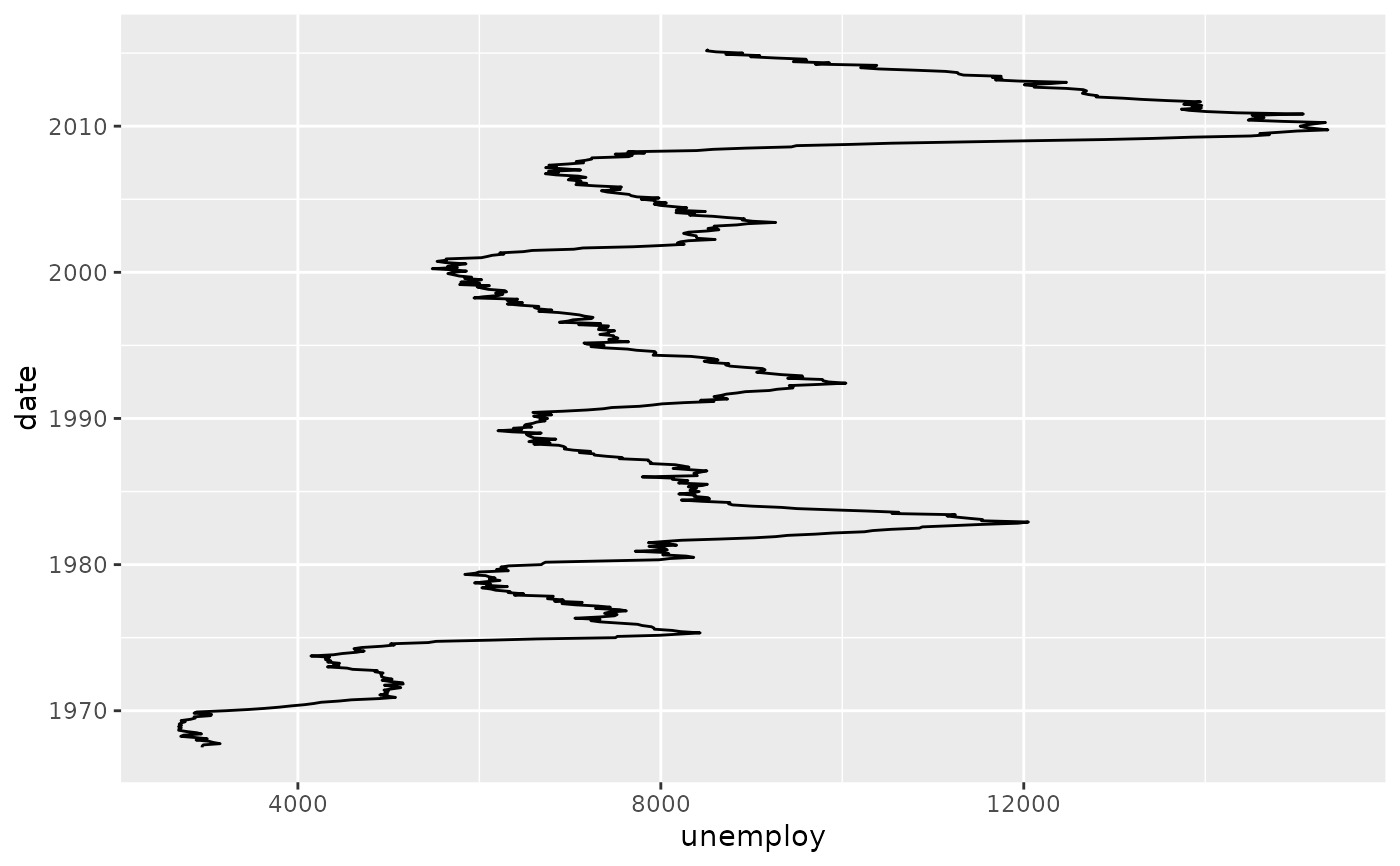
 # You can get a timeseries that run vertically by setting the orientation
ggplot(economics, aes(unemploy, date)) + geom_line(orientation = "y")
# You can get a timeseries that run vertically by setting the orientation
ggplot(economics, aes(unemploy, date)) + geom_line(orientation = "y")
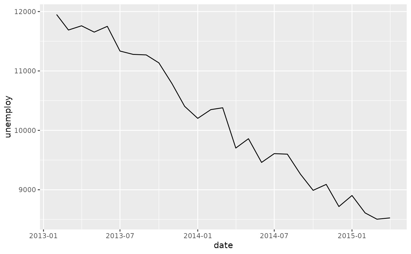
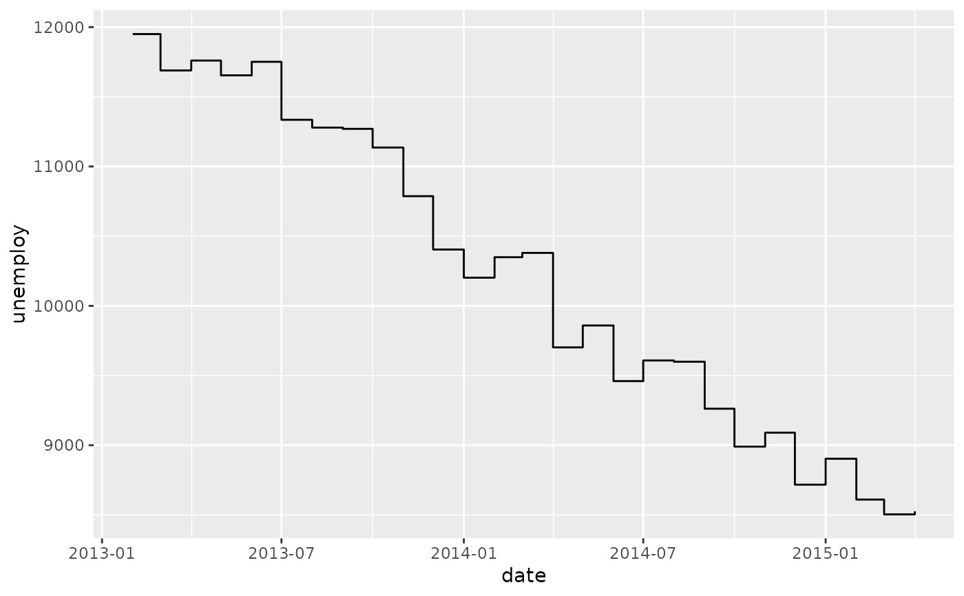
 # geom_step() is useful when you want to highlight exactly when
# the y value changes
recent <- economics[economics$date > as.Date("2013-01-01"), ]
ggplot(recent, aes(date, unemploy)) + geom_line()
# geom_step() is useful when you want to highlight exactly when
# the y value changes
recent <- economics[economics$date > as.Date("2013-01-01"), ]
ggplot(recent, aes(date, unemploy)) + geom_line()
 ggplot(recent, aes(date, unemploy)) + geom_step()
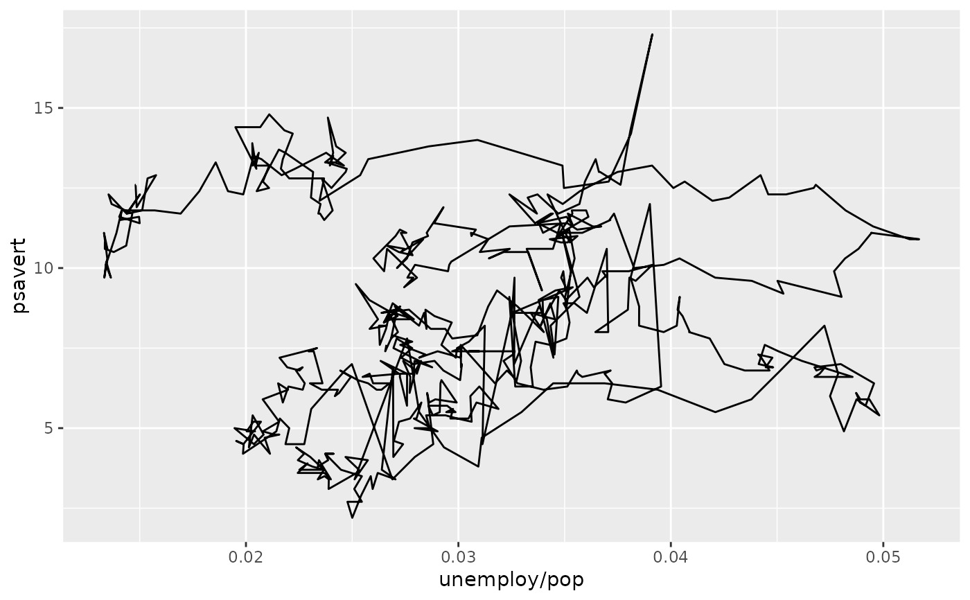
 # geom_path lets you explore how two variables are related over time,
# e.g. unemployment and personal savings rate
m <- ggplot(economics, aes(unemploy/pop, psavert))
m + geom_path()
# geom_path lets you explore how two variables are related over time,
# e.g. unemployment and personal savings rate
m <- ggplot(economics, aes(unemploy/pop, psavert))
m + geom_path()
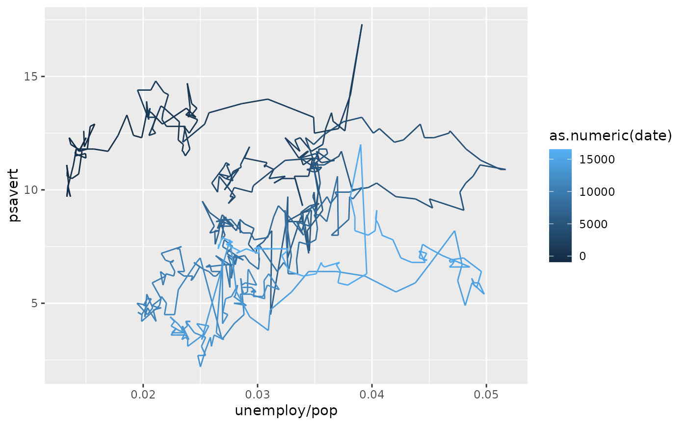
 m + geom_path(aes(colour = as.numeric(date)))
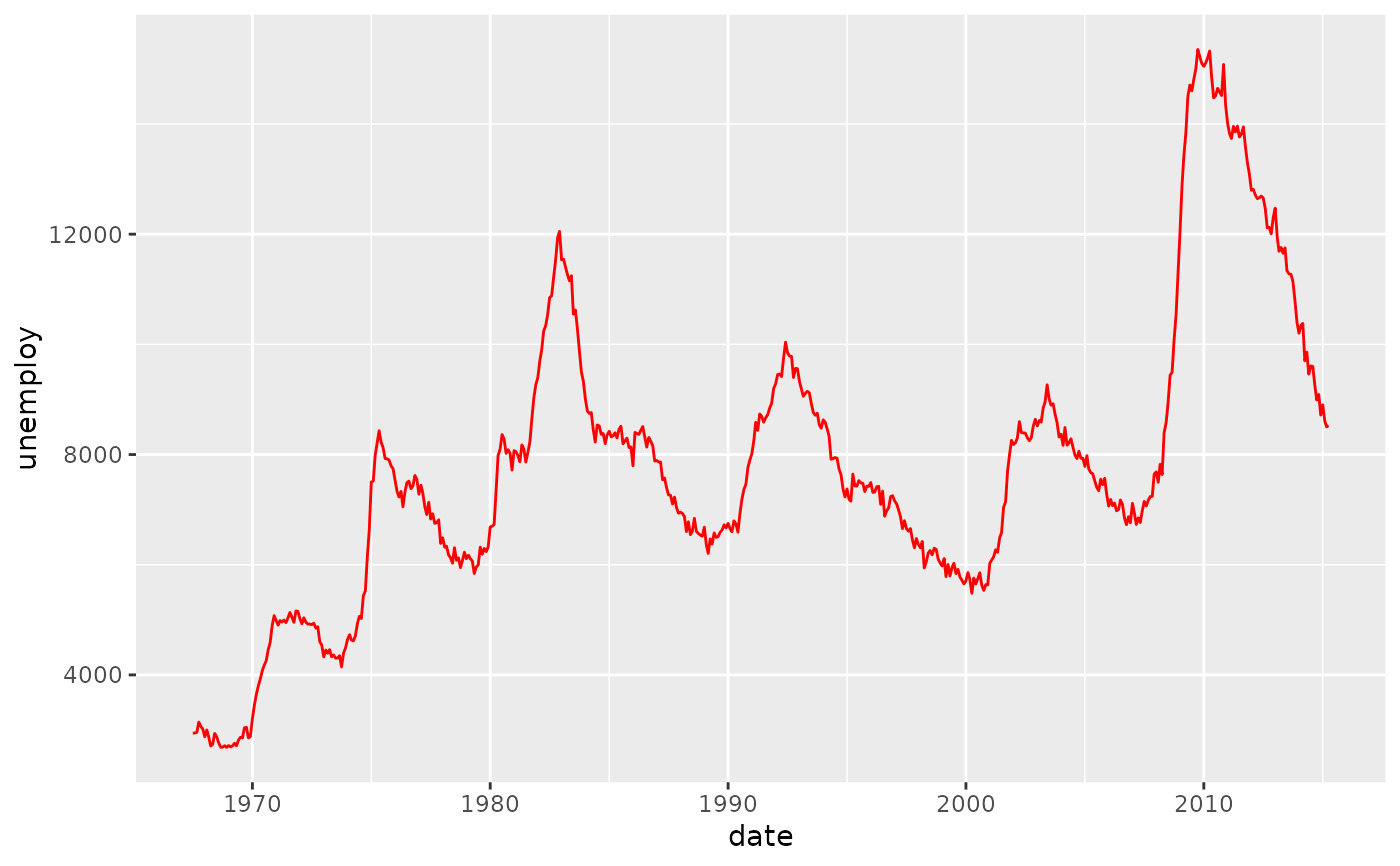
 # Changing parameters ----------------------------------------------
ggplot(economics, aes(date, unemploy)) +
geom_line(colour = "red")
# Changing parameters ----------------------------------------------
ggplot(economics, aes(date, unemploy)) +
geom_line(colour = "red")
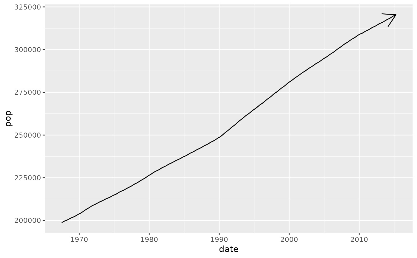
 # Use the arrow parameter to add an arrow to the line
# See ?arrow for more details
c <- ggplot(economics, aes(x = date, y = pop))
c + geom_line(arrow = arrow())
# Use the arrow parameter to add an arrow to the line
# See ?arrow for more details
c <- ggplot(economics, aes(x = date, y = pop))
c + geom_line(arrow = arrow())
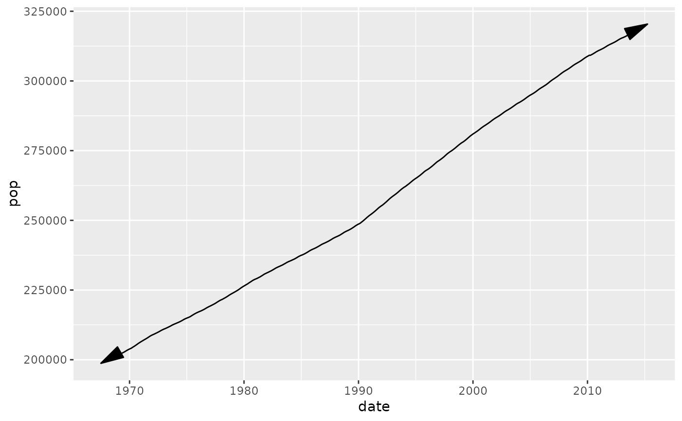
 c + geom_line(
arrow = arrow(angle = 15, ends = "both", type = "closed")
)
c + geom_line(
arrow = arrow(angle = 15, ends = "both", type = "closed")
)
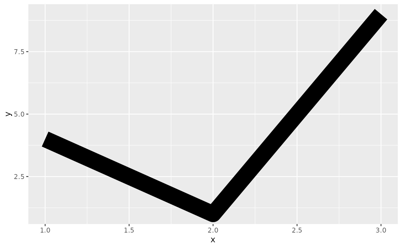
 # Control line join parameters
df <- data.frame(x = 1:3, y = c(4, 1, 9))
base <- ggplot(df, aes(x, y))
base + geom_path(linewidth = 10)
# Control line join parameters
df <- data.frame(x = 1:3, y = c(4, 1, 9))
base <- ggplot(df, aes(x, y))
base + geom_path(linewidth = 10)
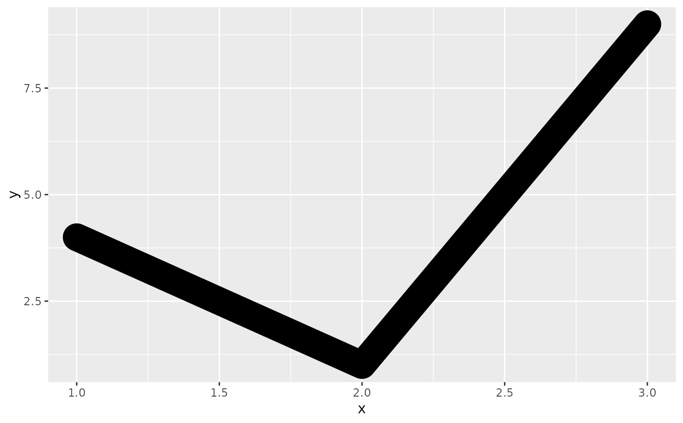
 base + geom_path(linewidth = 10, lineend = "round")
 base + geom_path(linewidth = 10, linejoin = "mitre", lineend = "butt")
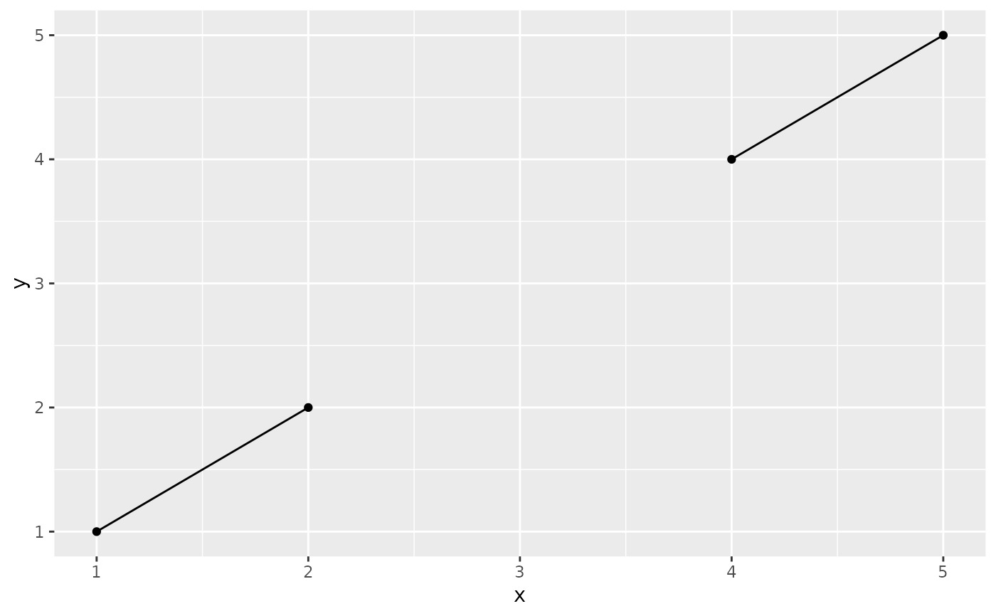
 # You can use NAs to break the line.
df <- data.frame(x = 1:5, y = c(1, 2, NA, 4, 5))
ggplot(df, aes(x, y)) + geom_point() + geom_line()
#> Warning: Removed 1 rows containing missing values (`geom_point()`).
# You can use NAs to break the line.
df <- data.frame(x = 1:5, y = c(1, 2, NA, 4, 5))
ggplot(df, aes(x, y)) + geom_point() + geom_line()
#> Warning: Removed 1 rows containing missing values (`geom_point()`).
 # \donttest{
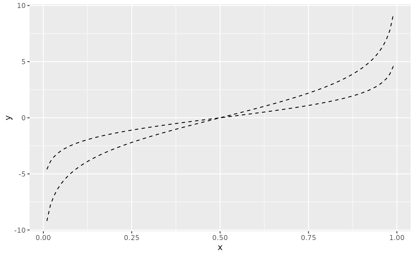
# Setting line type vs colour/size
# Line type needs to be applied to a line as a whole, so it can
# not be used with colour or size that vary across a line
x <- seq(0.01, .99, length.out = 100)
df <- data.frame(
x = rep(x, 2),
y = c(qlogis(x), 2 * qlogis(x)),
group = rep(c("a","b"),
each = 100)
)
p <- ggplot(df, aes(x=x, y=y, group=group))
# These work
p + geom_line(linetype = 2)
# \donttest{
# Setting line type vs colour/size
# Line type needs to be applied to a line as a whole, so it can
# not be used with colour or size that vary across a line
x <- seq(0.01, .99, length.out = 100)
df <- data.frame(
x = rep(x, 2),
y = c(qlogis(x), 2 * qlogis(x)),
group = rep(c("a","b"),
each = 100)
)
p <- ggplot(df, aes(x=x, y=y, group=group))
# These work
p + geom_line(linetype = 2)
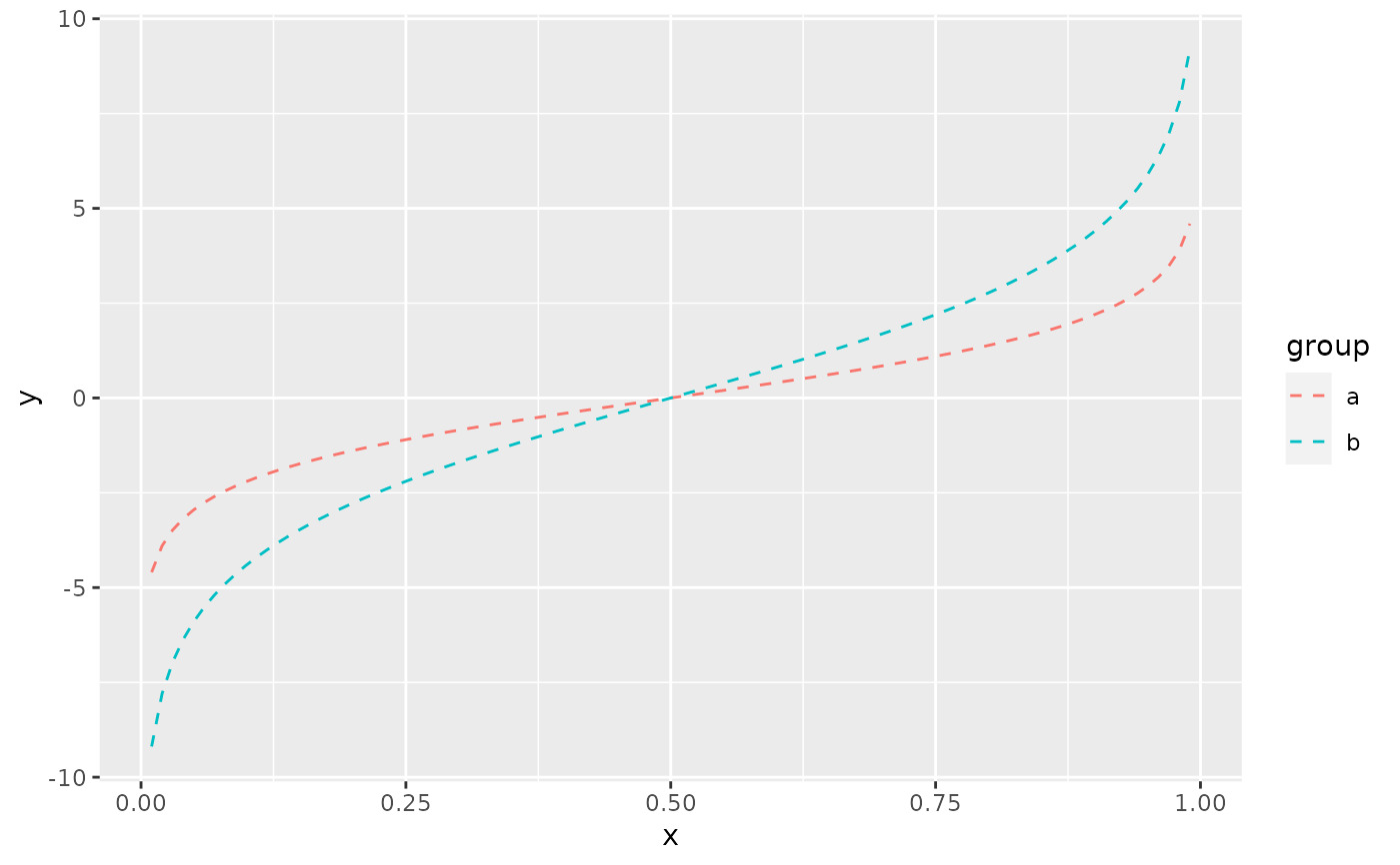
 p + geom_line(aes(colour = group), linetype = 2)
 p + geom_line(aes(colour = x))
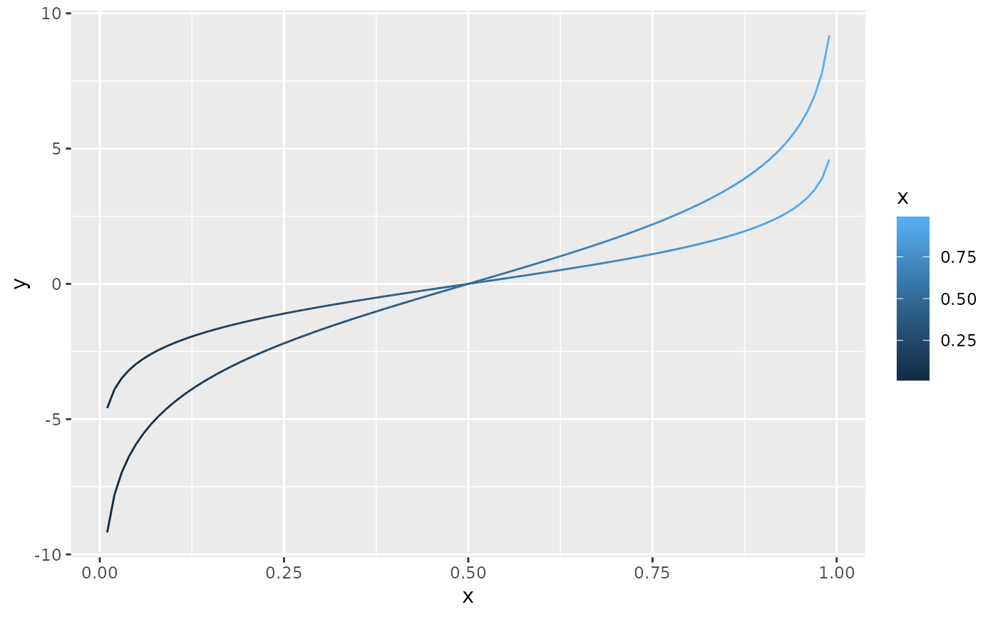 # But this doesn't
should_stop(p + geom_line(aes(colour = x), linetype=2))
# }
# But this doesn't
should_stop(p + geom_line(aes(colour = x), linetype=2))
# }
相关用法
- R ggplot2 geom_point 积分
- R ggplot2 geom_polygon 多边形
- R ggplot2 geom_qq 分位数-分位数图
- R ggplot2 geom_spoke 由位置、方向和距离参数化的线段
- R ggplot2 geom_quantile 分位数回归
- R ggplot2 geom_text 文本
- R ggplot2 geom_ribbon 函数区和面积图
- R ggplot2 geom_boxplot 盒须图(Tukey 风格)
- R ggplot2 geom_hex 二维箱计数的六边形热图
- R ggplot2 geom_bar 条形图
- R ggplot2 geom_bin_2d 二维 bin 计数热图
- R ggplot2 geom_jitter 抖动点
- R ggplot2 geom_linerange 垂直间隔:线、横线和误差线
- R ggplot2 geom_blank 什么也不画
- R ggplot2 geom_violin 小提琴情节
- R ggplot2 geom_dotplot 点图
- R ggplot2 geom_errorbarh 水平误差线
- R ggplot2 geom_function 将函数绘制为连续曲线
- R ggplot2 geom_histogram 直方图和频数多边形
- R ggplot2 geom_tile 矩形
- R ggplot2 geom_segment 线段和曲线
- R ggplot2 geom_density_2d 二维密度估计的等值线
- R ggplot2 geom_map 参考Map中的多边形
- R ggplot2 geom_density 平滑密度估计
- R ggplot2 geom_abline 参考线:水平、垂直和对角线
注:本文由纯净天空筛选整理自Hadley Wickham等大神的英文原创作品 Connect observations。非经特殊声明,原始代码版权归原作者所有,本译文未经允许或授权,请勿转载或复制。