使用 MASS::kde2d() 执行 2D 核密度估计并用轮廓显示结果。这对于处理过度绘图很有用。这是 geom_density() 的 2D 版本。 geom_density_2d() 绘制等高线,geom_density_2d_filled() 绘制填充等高线带。
用法
geom_density_2d(
  mapping = NULL,
  data = NULL,
  stat = "density_2d",
  position = "identity",
  ...,
  contour_var = "density",
  lineend = "butt",
  linejoin = "round",
  linemitre = 10,
  na.rm = FALSE,
  show.legend = NA,
  inherit.aes = TRUE
)

geom_density_2d_filled(
  mapping = NULL,
  data = NULL,
  stat = "density_2d_filled",
  position = "identity",
  ...,
  contour_var = "density",
  na.rm = FALSE,
  show.legend = NA,
  inherit.aes = TRUE
)

stat_density_2d(
  mapping = NULL,
  data = NULL,
  geom = "density_2d",
  position = "identity",
  ...,
  contour = TRUE,
  contour_var = "density",
  n = 100,
  h = NULL,
  adjust = c(1, 1),
  na.rm = FALSE,
  show.legend = NA,
  inherit.aes = TRUE
)

stat_density_2d_filled(
  mapping = NULL,
  data = NULL,
  geom = "density_2d_filled",
  position = "identity",
  ...,
  contour = TRUE,
  contour_var = "density",
  n = 100,
  h = NULL,
  adjust = c(1, 1),
  na.rm = FALSE,
  show.legend = NA,
  inherit.aes = TRUE
)
参数
- mapping
-
由
aes()创建的一组美学映射。如果指定且inherit.aes = TRUE(默认),它将与绘图顶层的默认映射组合。如果没有绘图映射,则必须提供mapping。 - data
-
该层要显示的数据。有以下三种选择:
如果默认为
NULL,则数据继承自ggplot()调用中指定的绘图数据。data.frame或其他对象将覆盖绘图数据。所有对象都将被强化以生成 DataFrame 。请参阅fortify()将为其创建变量。将使用单个参数(绘图数据)调用
function。返回值必须是data.frame,并将用作图层数据。可以从formula创建function(例如~ head(.x, 10))。 - position
-
位置调整,可以是命名调整的字符串(例如
"jitter"使用position_jitter),也可以是调用位置调整函数的结果。如果需要更改调整设置,请使用后者。 - ...
-
参数传递给
geom_contourbinwidth-
轮廓箱的宽度。被
bins覆盖。 bins-
轮廓箱的数量。被
breaks覆盖。 breaks-
之一:
-
用于设置轮廓中断的数值向量
-
该函数将数据范围和 binwidth 作为输入,并返回中断作为输出。可以根据公式创建函数(例如 ~ fullseq(.x, .y))。
覆盖
binwidth和bins。默认情况下,这是一个长度为 10 且带有pretty()中断的向量。 -
- contour_var
-
标识轮廓变量的字符串。可以是
"density"、"ndensity"或"count"之一。有关详细信息,请参阅有关计算变量的部分。 - lineend
-
线端样式(圆形、对接、方形)。
- linejoin
-
线连接样式(圆形、斜接、斜角)。
- linemitre
-
线斜接限制(数量大于 1)。
- na.rm
-
如果
FALSE,则默认缺失值将被删除并带有警告。如果TRUE,缺失值将被静默删除。 - show.legend
-
合乎逻辑的。该层是否应该包含在图例中?
NA(默认值)包括是否映射了任何美学。FALSE从不包含,而TRUE始终包含。它也可以是一个命名的逻辑向量,以精细地选择要显示的美学。 - inherit.aes
-
如果
FALSE,则覆盖默认美学,而不是与它们组合。这对于定义数据和美观的辅助函数最有用,并且不应继承默认绘图规范的行为,例如borders()。 - geom, stat
-
用于覆盖
geom_density_2d()和stat_density_2d()之间的默认连接。 - contour
-
如果
TRUE,绘制二维密度估计结果的轮廓。 - n
-
每个方向上的网格点数。
- h
-
带宽(长度为二的向量)。如果
NULL,则使用MASS::bandwidth.nrd()估计。 - adjust
-
如果'h' 是'NULL',则使用乘法带宽调整。这使得在仍然使用带宽估计器的同时调整带宽成为可能。例如
adjust = 1/2表示使用默认带宽的一半。
美学
geom_density_2d() 理解以下美学(所需的美学以粗体显示):
-
x -
y -
alpha -
colour -
group -
linetype -
linewidth
在 vignette("ggplot2-specs") 中了解有关设置这些美学的更多信息。
geom_density_2d_filled() 理解以下美学(所需的美学以粗体显示):
-
x -
y -
alpha -
colour -
fill -
group -
linetype -
linewidth -
subgroup
在 vignette("ggplot2-specs") 中了解有关设置这些美学的更多信息。
计算变量
这些是由层的 'stat' 部分计算的,可以使用 delayed evaluation 访问。 stat_density_2d() 和 stat_density_2d_filled() 根据轮廓绘制是否打开或关闭来计算不同的变量。当轮廓关闭(contour = FALSE)时,两个统计数据的行为相同,并且提供以下变量:
-
after_stat(density)
密度估计。 -
after_stat(ndensity)
密度估计,缩放至最大值 1。 -
after_stat(count)
密度估计 * 组中的观察数。 -
after_stat(n)
每组中的观察数。
启用轮廓绘制 ( contour = TRUE ) 后,在获得密度估计值后运行 stat_contour() 或 stat_contour_filled()(分别针对轮廓线或轮廓带),并且计算的变量由这些统计数据确定。针对轮廓绘制之前获得的三种类型的密度估计值之一( density 、 ndensity 和 count )计算轮廓。应使用其中哪一个由contour_var 参数确定。
也可以看看
geom_contour() 、 geom_contour_filled() 了解如何绘制轮廓的信息; geom_bin2d() 另一种处理过度绘制的方法。
例子
m <- ggplot(faithful, aes(x = eruptions, y = waiting)) +
geom_point() +
xlim(0.5, 6) +
ylim(40, 110)
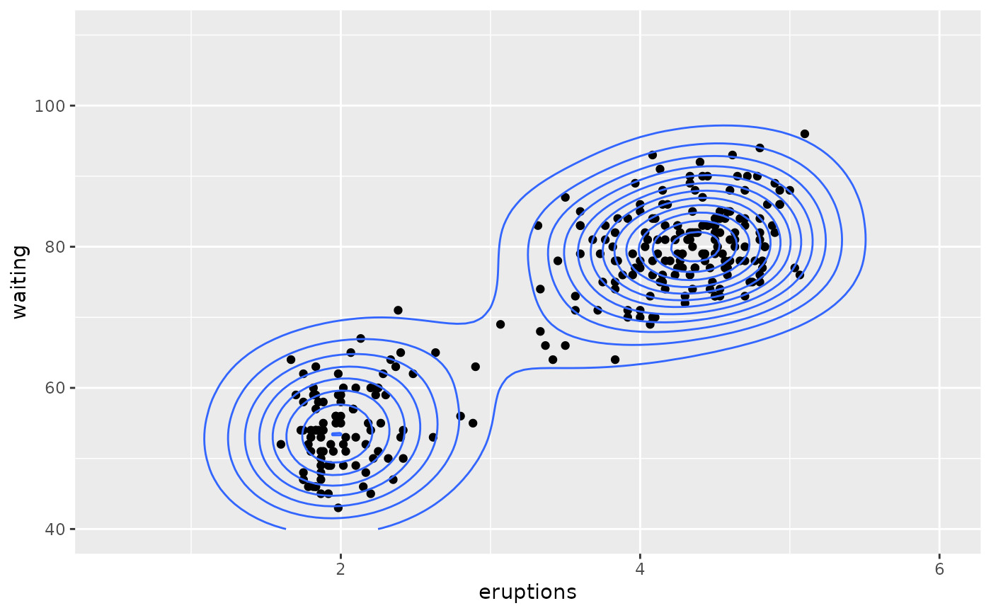
# contour lines
m + geom_density_2d()
 # \donttest{
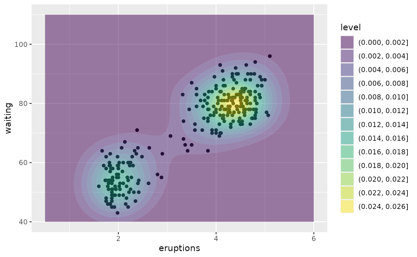
# contour bands
m + geom_density_2d_filled(alpha = 0.5)
# \donttest{
# contour bands
m + geom_density_2d_filled(alpha = 0.5)
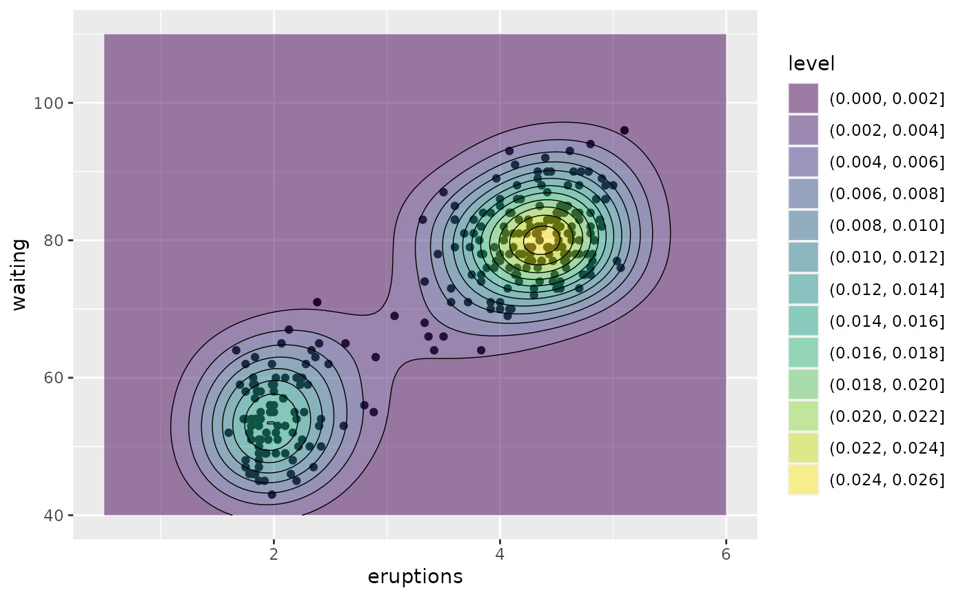
 # contour bands and contour lines
m + geom_density_2d_filled(alpha = 0.5) +
geom_density_2d(linewidth = 0.25, colour = "black")
# contour bands and contour lines
m + geom_density_2d_filled(alpha = 0.5) +
geom_density_2d(linewidth = 0.25, colour = "black")
 set.seed(4393)
dsmall <- diamonds[sample(nrow(diamonds), 1000), ]
d <- ggplot(dsmall, aes(x, y))
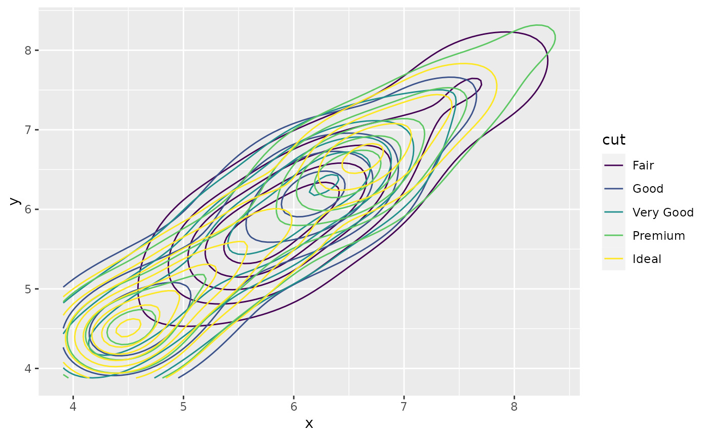
# If you map an aesthetic to a categorical variable, you will get a
# set of contours for each value of that variable
d + geom_density_2d(aes(colour = cut))
set.seed(4393)
dsmall <- diamonds[sample(nrow(diamonds), 1000), ]
d <- ggplot(dsmall, aes(x, y))
# If you map an aesthetic to a categorical variable, you will get a
# set of contours for each value of that variable
d + geom_density_2d(aes(colour = cut))
 # If you draw filled contours across multiple facets, the same bins are
# used across all facets
d + geom_density_2d_filled() + facet_wrap(vars(cut))
# If you draw filled contours across multiple facets, the same bins are
# used across all facets
d + geom_density_2d_filled() + facet_wrap(vars(cut))
 # If you want to make sure the peak intensity is the same in each facet,
# use `contour_var = "ndensity"`.
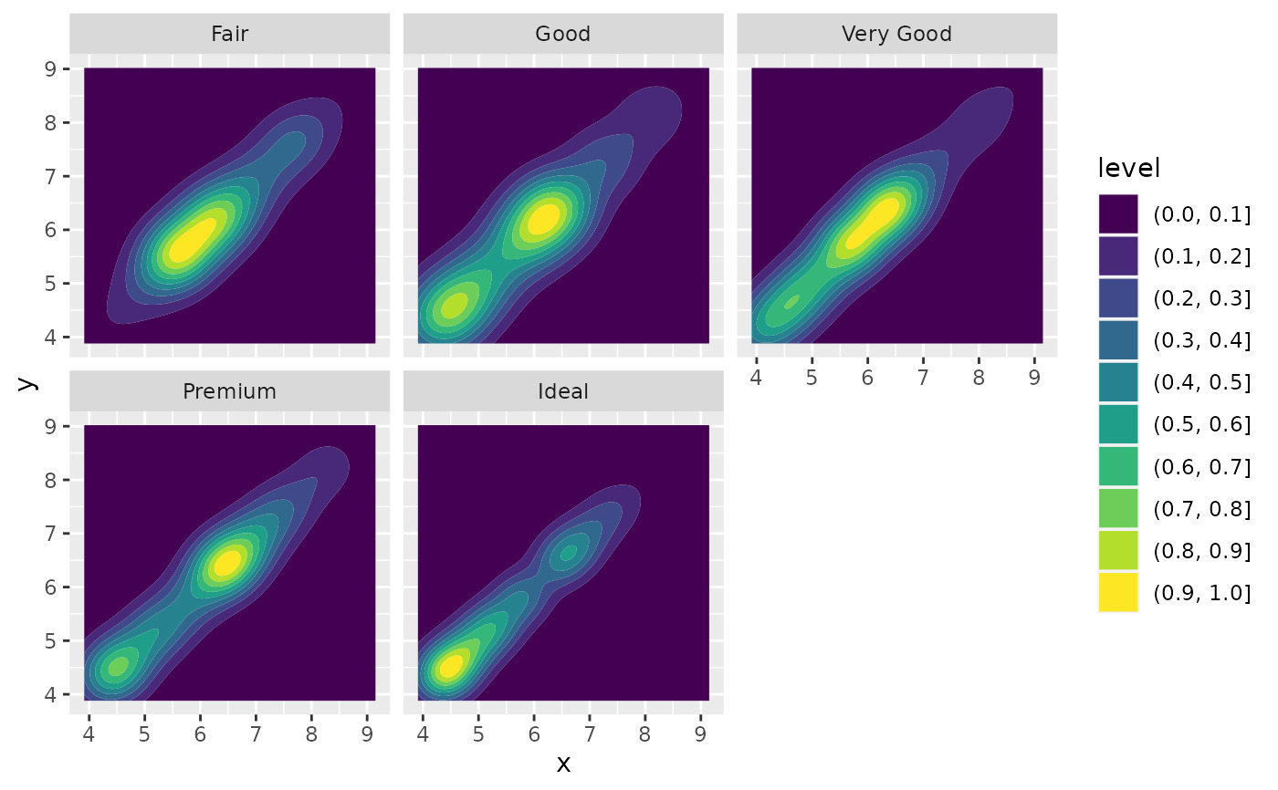
d + geom_density_2d_filled(contour_var = "ndensity") + facet_wrap(vars(cut))
# If you want to make sure the peak intensity is the same in each facet,
# use `contour_var = "ndensity"`.
d + geom_density_2d_filled(contour_var = "ndensity") + facet_wrap(vars(cut))
 # If you want to scale intensity by the number of observations in each group,
# use `contour_var = "count"`.
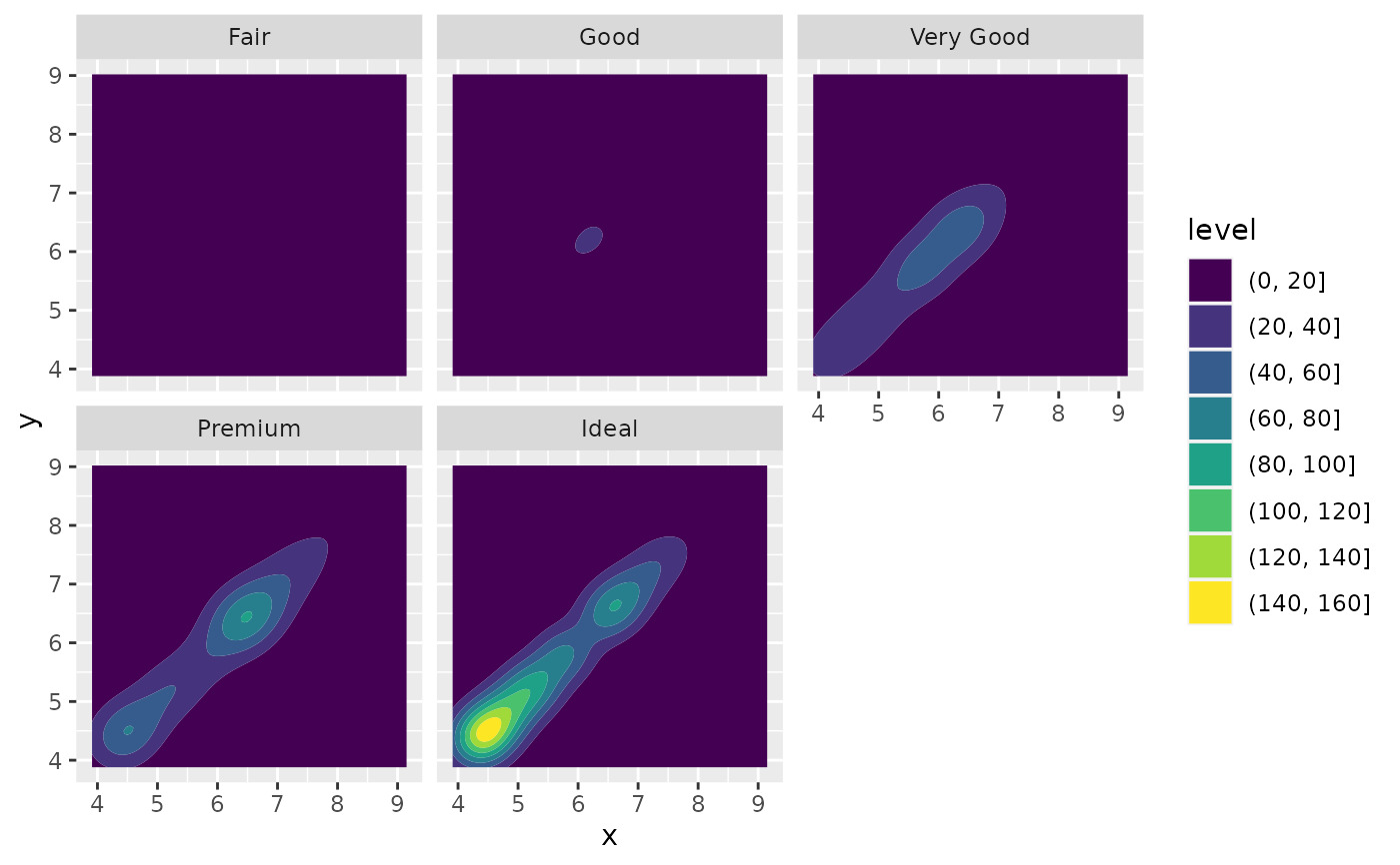
d + geom_density_2d_filled(contour_var = "count") + facet_wrap(vars(cut))
# If you want to scale intensity by the number of observations in each group,
# use `contour_var = "count"`.
d + geom_density_2d_filled(contour_var = "count") + facet_wrap(vars(cut))
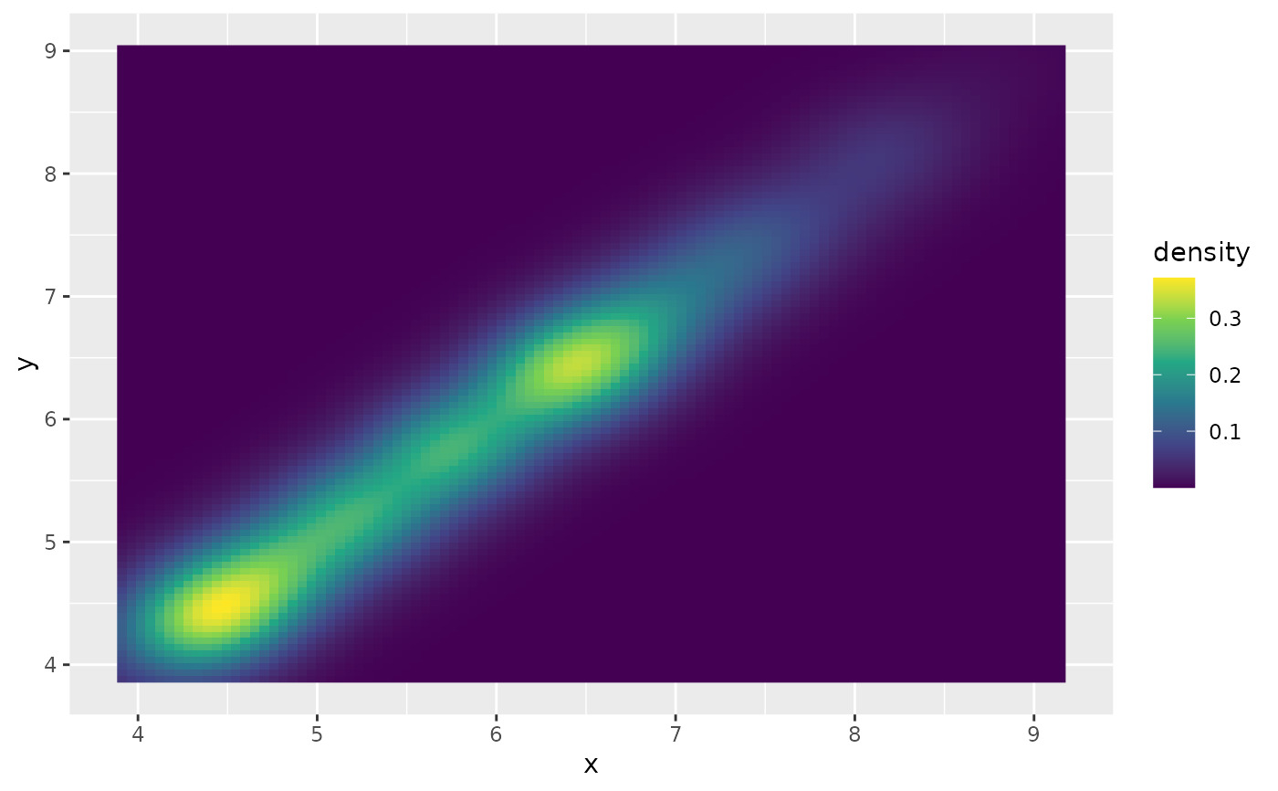
 # If we turn contouring off, we can use other geoms, such as tiles:
d + stat_density_2d(
geom = "raster",
aes(fill = after_stat(density)),
contour = FALSE
) + scale_fill_viridis_c()
# If we turn contouring off, we can use other geoms, such as tiles:
d + stat_density_2d(
geom = "raster",
aes(fill = after_stat(density)),
contour = FALSE
) + scale_fill_viridis_c()
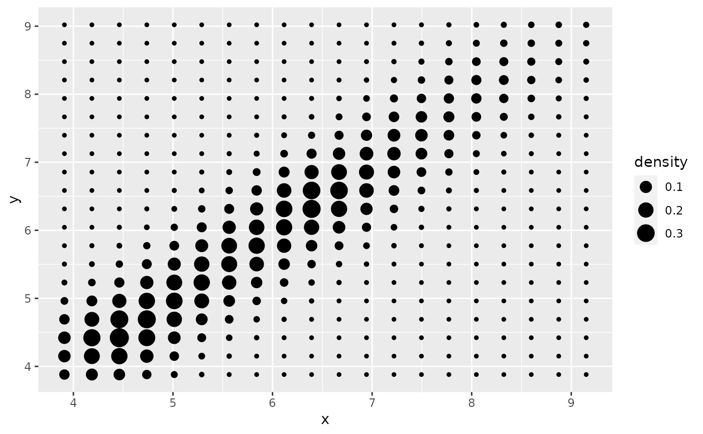
 # Or points:
d + stat_density_2d(geom = "point", aes(size = after_stat(density)), n = 20, contour = FALSE)
# Or points:
d + stat_density_2d(geom = "point", aes(size = after_stat(density)), n = 20, contour = FALSE)
 # }
# }
相关用法
- R ggplot2 geom_density 平滑密度估计
- R ggplot2 geom_dotplot 点图
- R ggplot2 geom_qq 分位数-分位数图
- R ggplot2 geom_spoke 由位置、方向和距离参数化的线段
- R ggplot2 geom_quantile 分位数回归
- R ggplot2 geom_text 文本
- R ggplot2 geom_ribbon 函数区和面积图
- R ggplot2 geom_boxplot 盒须图(Tukey 风格)
- R ggplot2 geom_hex 二维箱计数的六边形热图
- R ggplot2 geom_bar 条形图
- R ggplot2 geom_bin_2d 二维 bin 计数热图
- R ggplot2 geom_jitter 抖动点
- R ggplot2 geom_point 积分
- R ggplot2 geom_linerange 垂直间隔:线、横线和误差线
- R ggplot2 geom_blank 什么也不画
- R ggplot2 geom_path 连接观察结果
- R ggplot2 geom_violin 小提琴情节
- R ggplot2 geom_errorbarh 水平误差线
- R ggplot2 geom_function 将函数绘制为连续曲线
- R ggplot2 geom_polygon 多边形
- R ggplot2 geom_histogram 直方图和频数多边形
- R ggplot2 geom_tile 矩形
- R ggplot2 geom_segment 线段和曲线
- R ggplot2 geom_map 参考Map中的多边形
- R ggplot2 geom_abline 参考线:水平、垂直和对角线
注:本文由纯净天空筛选整理自Hadley Wickham等大神的英文原创作品 Contours of a 2D density estimate。非经特殊声明,原始代码版权归原作者所有,本译文未经允许或授权,请勿转载或复制。