多边形与路径(由 geom_path() 绘制)非常相似,只是起点和终点是相连的,并且内部由 fill 着色。 group 美学决定了哪些案例连接在一起形成多边形。从 R 3.6 及更高版本开始,可以通过提供子组美感来绘制带孔的多边形,该子组美感可将外环点与说明多边形中的孔的点区分开来。
用法
geom_polygon(
  mapping = NULL,
  data = NULL,
  stat = "identity",
  position = "identity",
  rule = "evenodd",
  ...,
  na.rm = FALSE,
  show.legend = NA,
  inherit.aes = TRUE
)
参数
- mapping
-
由
aes()创建的一组美学映射。如果指定且inherit.aes = TRUE(默认),它将与绘图顶层的默认映射组合。如果没有绘图映射,则必须提供mapping。 - data
-
该层要显示的数据。有以下三种选择:
如果默认为
NULL,则数据继承自ggplot()调用中指定的绘图数据。data.frame或其他对象将覆盖绘图数据。所有对象都将被强化以生成 DataFrame 。请参阅fortify()将为其创建变量。将使用单个参数(绘图数据)调用
function。返回值必须是data.frame,并将用作图层数据。可以从formula创建function(例如~ head(.x, 10))。 - stat
-
用于该层数据的统计变换,可以作为
ggprotoGeom子类,也可以作为命名去掉stat_前缀的统计数据的字符串(例如"count"而不是"stat_count") - position
-
位置调整,可以是命名调整的字符串(例如
"jitter"使用position_jitter),也可以是调用位置调整函数的结果。如果需要更改调整设置,请使用后者。 - rule
-
"evenodd"或"winding"。如果正在绘制带孔的多边形(使用subgroup美学),则此参数定义如何解释孔坐标。有关说明,请参阅grid::pathGrob()中的示例。 - ...
-
其他参数传递给
layer()。这些通常是美学,用于将美学设置为固定值,例如colour = "red"或size = 3。它们也可能是配对的 geom/stat 的参数。 - na.rm
-
如果
FALSE,则默认缺失值将被删除并带有警告。如果TRUE,缺失值将被静默删除。 - show.legend
-
合乎逻辑的。该层是否应该包含在图例中?
NA(默认值)包括是否映射了任何美学。FALSE从不包含,而TRUE始终包含。它也可以是一个命名的逻辑向量,以精细地选择要显示的美学。 - inherit.aes
-
如果
FALSE,则覆盖默认美学,而不是与它们组合。这对于定义数据和美观的辅助函数最有用,并且不应继承默认绘图规范的行为,例如borders()。
美学
geom_polygon() 理解以下美学(所需的美学以粗体显示):
-
x -
y -
alpha -
colour -
fill -
group -
linetype -
linewidth -
subgroup
在 vignette("ggplot2-specs") 中了解有关设置这些美学的更多信息。
也可以看看
geom_path() 表示未填充的多边形,geom_ribbon() 表示锚定在 x 轴上的多边形
例子
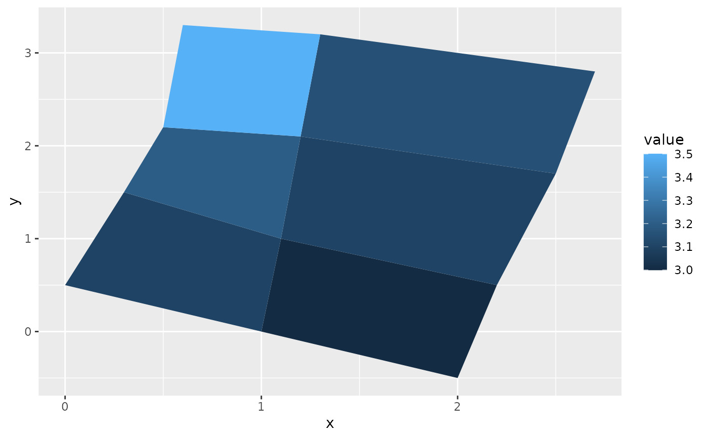
# When using geom_polygon, you will typically need two data frames:
# one contains the coordinates of each polygon (positions), and the
# other the values associated with each polygon (values). An id
# variable links the two together
ids <- factor(c("1.1", "2.1", "1.2", "2.2", "1.3", "2.3"))
values <- data.frame(
id = ids,
value = c(3, 3.1, 3.1, 3.2, 3.15, 3.5)
)
positions <- data.frame(
id = rep(ids, each = 4),
x = c(2, 1, 1.1, 2.2, 1, 0, 0.3, 1.1, 2.2, 1.1, 1.2, 2.5, 1.1, 0.3,
0.5, 1.2, 2.5, 1.2, 1.3, 2.7, 1.2, 0.5, 0.6, 1.3),
y = c(-0.5, 0, 1, 0.5, 0, 0.5, 1.5, 1, 0.5, 1, 2.1, 1.7, 1, 1.5,
2.2, 2.1, 1.7, 2.1, 3.2, 2.8, 2.1, 2.2, 3.3, 3.2)
)
# Currently we need to manually merge the two together
datapoly <- merge(values, positions, by = c("id"))
p <- ggplot(datapoly, aes(x = x, y = y)) +
geom_polygon(aes(fill = value, group = id))
p
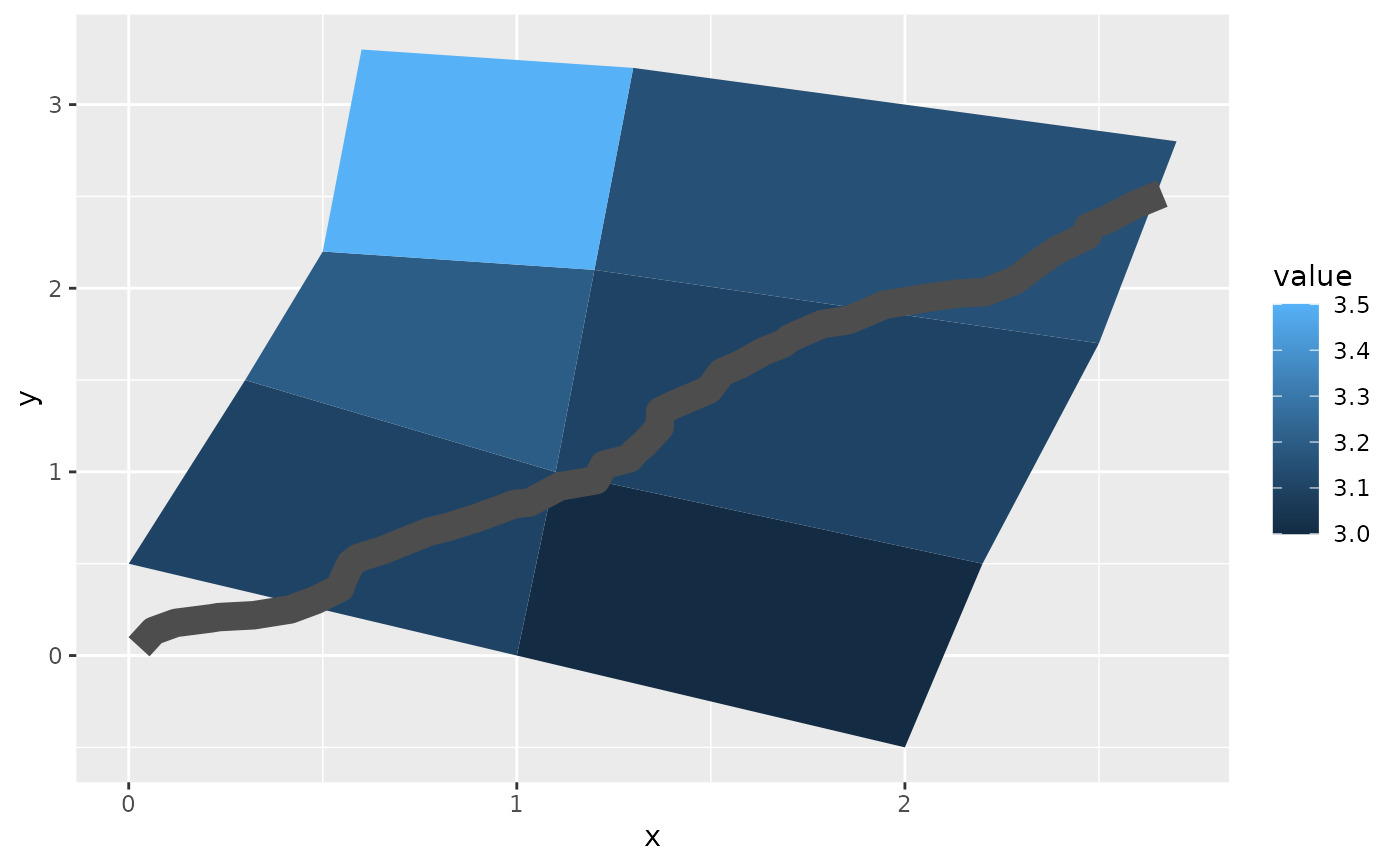
 # Which seems like a lot of work, but then it's easy to add on
# other features in this coordinate system, e.g.:
set.seed(1)
stream <- data.frame(
x = cumsum(runif(50, max = 0.1)),
y = cumsum(runif(50,max = 0.1))
)
p + geom_line(data = stream, colour = "grey30", linewidth = 5)
# Which seems like a lot of work, but then it's easy to add on
# other features in this coordinate system, e.g.:
set.seed(1)
stream <- data.frame(
x = cumsum(runif(50, max = 0.1)),
y = cumsum(runif(50,max = 0.1))
)
p + geom_line(data = stream, colour = "grey30", linewidth = 5)
 # And if the positions are in longitude and latitude, you can use
# coord_map to produce different map projections.
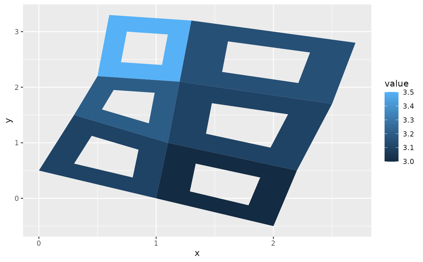
if (packageVersion("grid") >= "3.6") {
# As of R version 3.6 geom_polygon() supports polygons with holes
# Use the subgroup aesthetic to differentiate holes from the main polygon
holes <- do.call(rbind, lapply(split(datapoly, datapoly$id), function(df) {
df$x <- df$x + 0.5 * (mean(df$x) - df$x)
df$y <- df$y + 0.5 * (mean(df$y) - df$y)
df
}))
datapoly$subid <- 1L
holes$subid <- 2L
datapoly <- rbind(datapoly, holes)
p <- ggplot(datapoly, aes(x = x, y = y)) +
geom_polygon(aes(fill = value, group = id, subgroup = subid))
p
}
# And if the positions are in longitude and latitude, you can use
# coord_map to produce different map projections.
if (packageVersion("grid") >= "3.6") {
# As of R version 3.6 geom_polygon() supports polygons with holes
# Use the subgroup aesthetic to differentiate holes from the main polygon
holes <- do.call(rbind, lapply(split(datapoly, datapoly$id), function(df) {
df$x <- df$x + 0.5 * (mean(df$x) - df$x)
df$y <- df$y + 0.5 * (mean(df$y) - df$y)
df
}))
datapoly$subid <- 1L
holes$subid <- 2L
datapoly <- rbind(datapoly, holes)
p <- ggplot(datapoly, aes(x = x, y = y)) +
geom_polygon(aes(fill = value, group = id, subgroup = subid))
p
}
相关用法
- R ggplot2 geom_point 积分
- R ggplot2 geom_path 连接观察结果
- R ggplot2 geom_qq 分位数-分位数图
- R ggplot2 geom_spoke 由位置、方向和距离参数化的线段
- R ggplot2 geom_quantile 分位数回归
- R ggplot2 geom_text 文本
- R ggplot2 geom_ribbon 函数区和面积图
- R ggplot2 geom_boxplot 盒须图(Tukey 风格)
- R ggplot2 geom_hex 二维箱计数的六边形热图
- R ggplot2 geom_bar 条形图
- R ggplot2 geom_bin_2d 二维 bin 计数热图
- R ggplot2 geom_jitter 抖动点
- R ggplot2 geom_linerange 垂直间隔:线、横线和误差线
- R ggplot2 geom_blank 什么也不画
- R ggplot2 geom_violin 小提琴情节
- R ggplot2 geom_dotplot 点图
- R ggplot2 geom_errorbarh 水平误差线
- R ggplot2 geom_function 将函数绘制为连续曲线
- R ggplot2 geom_histogram 直方图和频数多边形
- R ggplot2 geom_tile 矩形
- R ggplot2 geom_segment 线段和曲线
- R ggplot2 geom_density_2d 二维密度估计的等值线
- R ggplot2 geom_map 参考Map中的多边形
- R ggplot2 geom_density 平滑密度估计
- R ggplot2 geom_abline 参考线:水平、垂直和对角线
注:本文由纯净天空筛选整理自Hadley Wickham等大神的英文原创作品 Polygons。非经特殊声明,原始代码版权归原作者所有,本译文未经允许或授权,请勿转载或复制。