这些几何图形将参考线(有时称为规则)添加到绘图中,无论是水平的、垂直的还是对角线的(由斜率和截距指定)。这些对于注释绘图很有用。
用法
geom_abline(
  mapping = NULL,
  data = NULL,
  ...,
  slope,
  intercept,
  na.rm = FALSE,
  show.legend = NA
)

geom_hline(
  mapping = NULL,
  data = NULL,
  ...,
  yintercept,
  na.rm = FALSE,
  show.legend = NA
)

geom_vline(
  mapping = NULL,
  data = NULL,
  ...,
  xintercept,
  na.rm = FALSE,
  show.legend = NA
)
参数
- mapping
-
由
aes()创建的一组美学映射。 - data
-
该层要显示的数据。有以下三种选择:
如果默认为
NULL,则数据继承自ggplot()调用中指定的绘图数据。data.frame或其他对象将覆盖绘图数据。所有对象都将被强化以生成 DataFrame 。请参阅fortify()将为其创建变量。将使用单个参数(绘图数据)调用
function。返回值必须是data.frame,并将用作图层数据。可以从formula创建function(例如~ head(.x, 10))。 - ...
-
其他参数传递给
layer()。这些通常是美学,用于将美学设置为固定值,例如colour = "red"或size = 3。它们也可能是配对的 geom/stat 的参数。 - na.rm
-
如果
FALSE,则默认缺失值将被删除并带有警告。如果TRUE,缺失值将被静默删除。 - show.legend
-
合乎逻辑的。该层是否应该包含在图例中?
NA(默认值)包括是否映射了任何美学。FALSE从不包含,而TRUE始终包含。它也可以是一个命名的逻辑向量,以精细地选择要显示的美学。 - xintercept, yintercept, slope, intercept
-
控制线位置的参数。如果设置了这些,则
data、mapping和show.legend将被覆盖。
细节
这些几何体的行为与其他几何体略有不同。您可以通过两种方式提供参数:作为图层函数的参数,或通过美学。如果您使用参数,例如geom_abline(intercept = 0, slope = 1) ,然后 geom 在幕后创建一个仅包含您提供的数据的新 DataFrame 。这意味着所有方面的线条都是相同的;如果您希望它们在各个方面有所不同,请自己构建 DataFrame 架并使用美学。
与大多数其他几何图形不同,这些几何图形不会从绘图默认继承美学,因为它们不理解绘图中通常设置的 x 和 y 美学。它们也不影响 x 和 y 尺度。
美学
这些几何体是使用 geom_line() 绘制的,因此它们支持相同的美学: alpha 、 colour 、 linetype 和 linewidth 。它们还各自具有控制线条位置的美学:
-
geom_vline():xintercept -
geom_hline():yintercept -
geom_abline():slope和intercept
也可以看看
有关向绘图添加直线段的更通用方法,请参阅geom_segment()。
例子
p <- ggplot(mtcars, aes(wt, mpg)) + geom_point()
# Fixed values
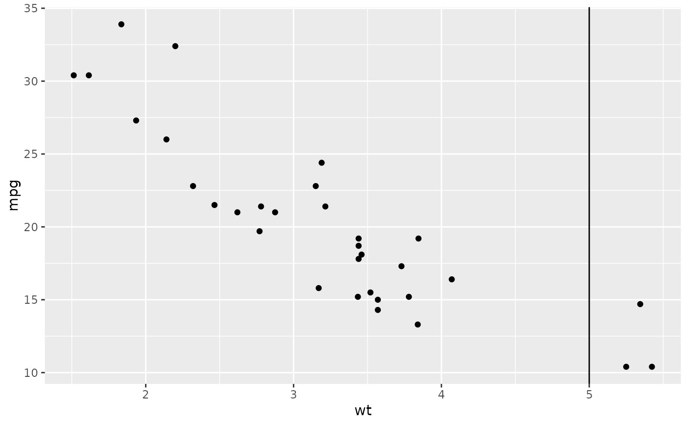
p + geom_vline(xintercept = 5)
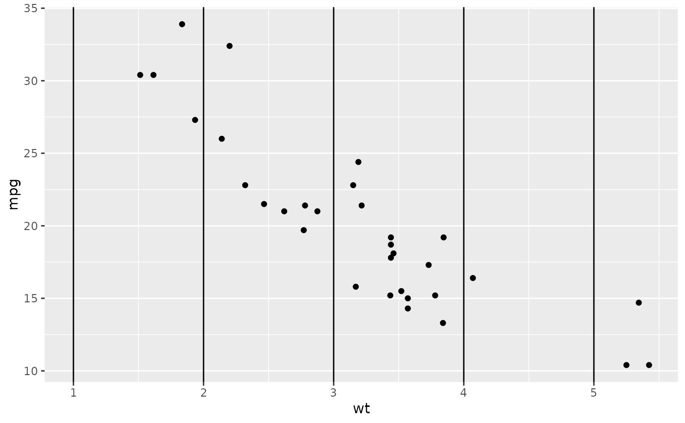
 p + geom_vline(xintercept = 1:5)
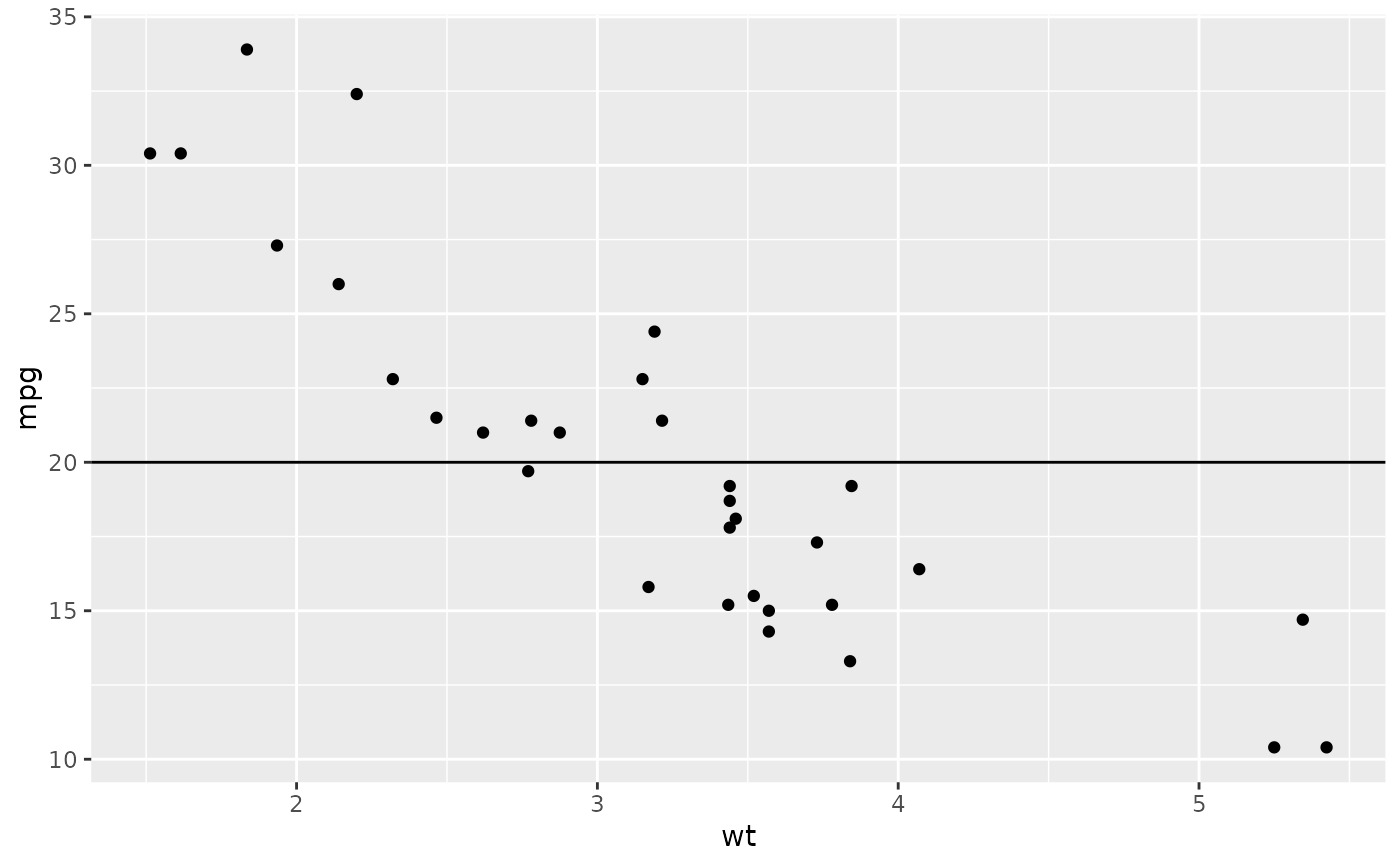
 p + geom_hline(yintercept = 20)
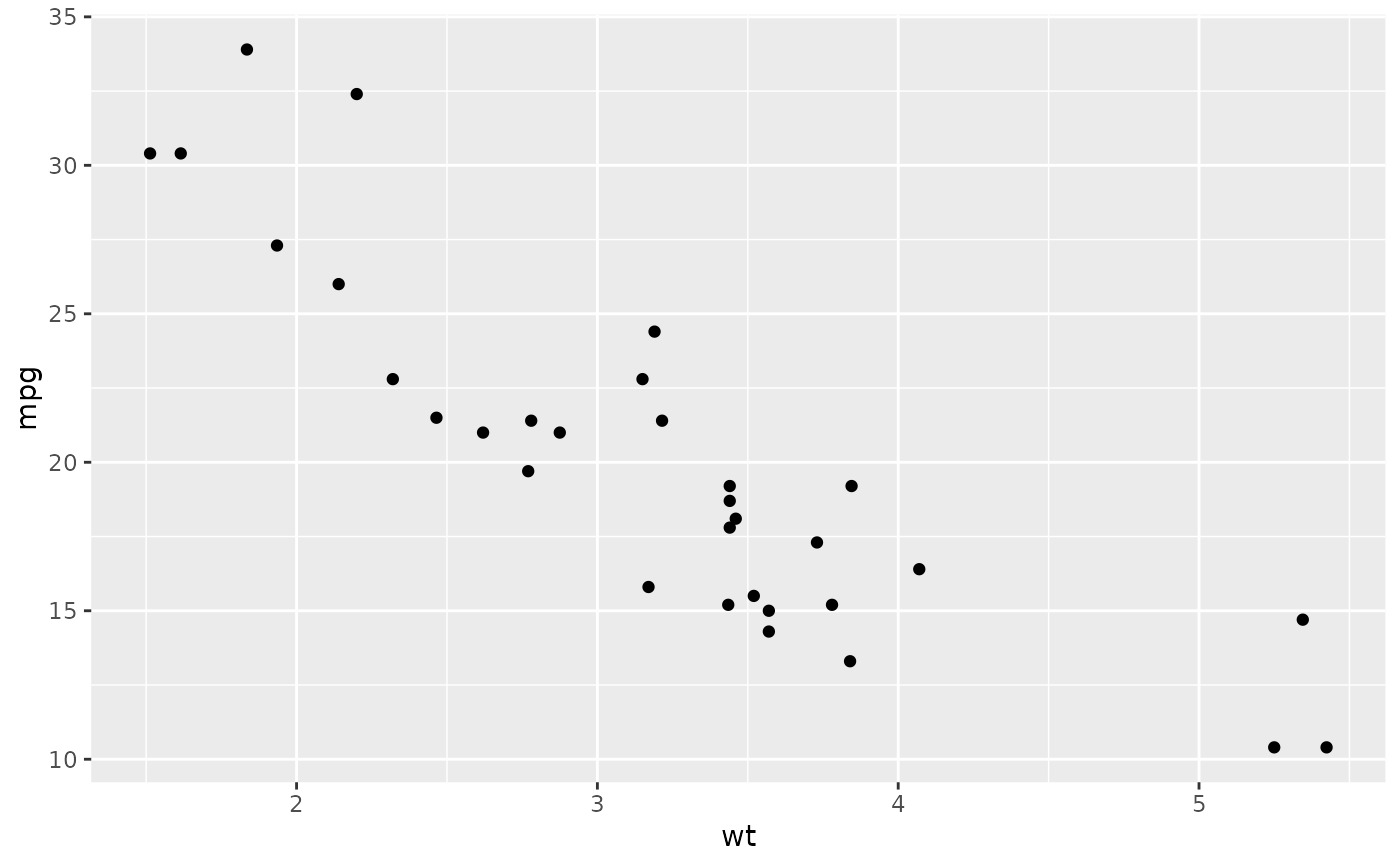
 p + geom_abline() # Can't see it - outside the range of the data
 p + geom_abline(intercept = 20)
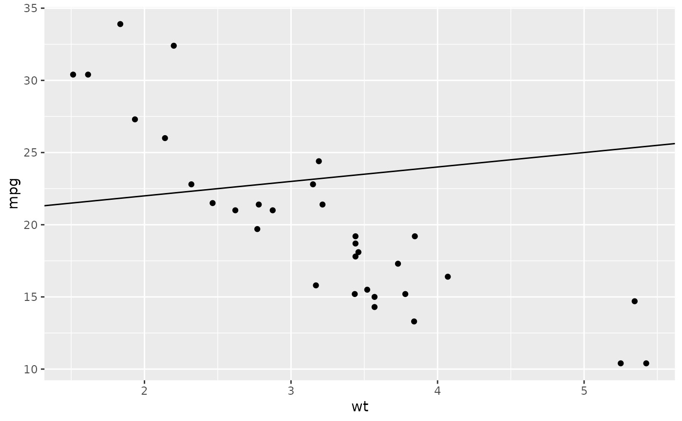 # Calculate slope and intercept of line of best fit
coef(lm(mpg ~ wt, data = mtcars))
#> (Intercept) wt
#> 37.285126 -5.344472
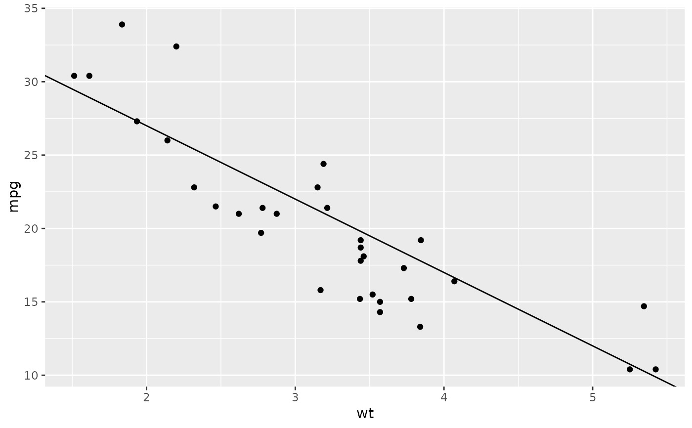
p + geom_abline(intercept = 37, slope = -5)
# Calculate slope and intercept of line of best fit
coef(lm(mpg ~ wt, data = mtcars))
#> (Intercept) wt
#> 37.285126 -5.344472
p + geom_abline(intercept = 37, slope = -5)
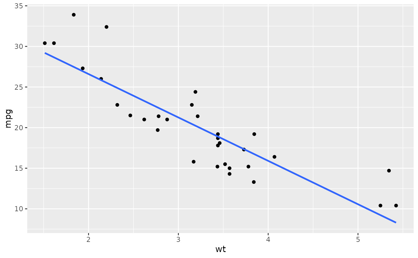
 # But this is easier to do with geom_smooth:
p + geom_smooth(method = "lm", se = FALSE)
#> `geom_smooth()` using formula = 'y ~ x'
# But this is easier to do with geom_smooth:
p + geom_smooth(method = "lm", se = FALSE)
#> `geom_smooth()` using formula = 'y ~ x'
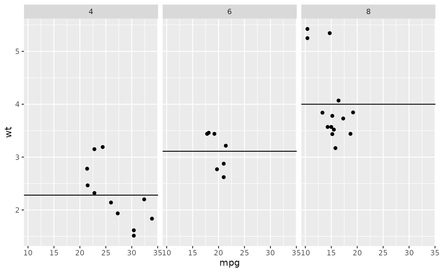
 # To show different lines in different facets, use aesthetics
p <- ggplot(mtcars, aes(mpg, wt)) +
geom_point() +
facet_wrap(~ cyl)
mean_wt <- data.frame(cyl = c(4, 6, 8), wt = c(2.28, 3.11, 4.00))
p + geom_hline(aes(yintercept = wt), mean_wt)
# To show different lines in different facets, use aesthetics
p <- ggplot(mtcars, aes(mpg, wt)) +
geom_point() +
facet_wrap(~ cyl)
mean_wt <- data.frame(cyl = c(4, 6, 8), wt = c(2.28, 3.11, 4.00))
p + geom_hline(aes(yintercept = wt), mean_wt)
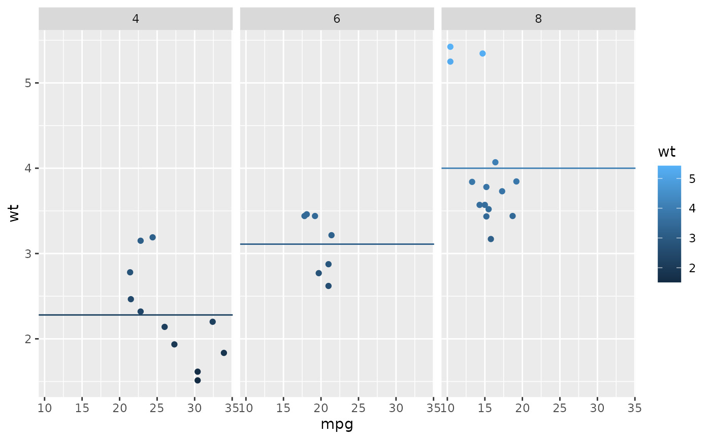
 # You can also control other aesthetics
ggplot(mtcars, aes(mpg, wt, colour = wt)) +
geom_point() +
geom_hline(aes(yintercept = wt, colour = wt), mean_wt) +
facet_wrap(~ cyl)
# You can also control other aesthetics
ggplot(mtcars, aes(mpg, wt, colour = wt)) +
geom_point() +
geom_hline(aes(yintercept = wt, colour = wt), mean_wt) +
facet_wrap(~ cyl)
相关用法
- R ggplot2 geom_qq 分位数-分位数图
- R ggplot2 geom_spoke 由位置、方向和距离参数化的线段
- R ggplot2 geom_quantile 分位数回归
- R ggplot2 geom_text 文本
- R ggplot2 geom_ribbon 函数区和面积图
- R ggplot2 geom_boxplot 盒须图(Tukey 风格)
- R ggplot2 geom_hex 二维箱计数的六边形热图
- R ggplot2 geom_bar 条形图
- R ggplot2 geom_bin_2d 二维 bin 计数热图
- R ggplot2 geom_jitter 抖动点
- R ggplot2 geom_point 积分
- R ggplot2 geom_linerange 垂直间隔:线、横线和误差线
- R ggplot2 geom_blank 什么也不画
- R ggplot2 geom_path 连接观察结果
- R ggplot2 geom_violin 小提琴情节
- R ggplot2 geom_dotplot 点图
- R ggplot2 geom_errorbarh 水平误差线
- R ggplot2 geom_function 将函数绘制为连续曲线
- R ggplot2 geom_polygon 多边形
- R ggplot2 geom_histogram 直方图和频数多边形
- R ggplot2 geom_tile 矩形
- R ggplot2 geom_segment 线段和曲线
- R ggplot2 geom_density_2d 二维密度估计的等值线
- R ggplot2 geom_map 参考Map中的多边形
- R ggplot2 geom_density 平滑密度估计
注:本文由纯净天空筛选整理自Hadley Wickham等大神的英文原创作品 Reference lines: horizontal, vertical, and diagonal。非经特殊声明,原始代码版权归原作者所有,本译文未经允许或授权,请勿转载或复制。