大多数aesthetics是从数据中找到的变量映射的。然而,有时您希望将映射延迟到渲染过程的后期。 ggplot2 具有三个阶段的数据,您可以从中映射美学,以及三个函数来控制在哪个阶段评估美学。
after_stat() 替换了使用 stat() 的旧方法,例如stat(density) ,或用 .. 包围变量名称,例如..density.. 。
用法
# These functions can be used inside the `aes()` function
# used as the `mapping` argument in layers, for example:
# geom_density(mapping = aes(y = after_stat(scaled)))

after_stat(x)

after_scale(x)

stage(start = NULL, after_stat = NULL, after_scale = NULL)
参数
- x
-
<
data-masking> 使用由统计 (after_stat()) 或图层美学 (after_scale()) 计算的变量的美学表达。 - start
-
<
data-masking> 使用图层数据变量的美学表达。 - after_stat
-
<
data-masking> 使用统计数据计算的变量的美学表达。 - after_scale
-
<
data-masking> 使用图层美学的美学表达。
分期
下面概述了评估的三个阶段以及如何控制美学评估。
第一阶段:直接输入
默认是在开始时使用用户提供的图层数据进行映射。如果你想直接从图层数据映射,你不应该做任何特殊的事情。这是可以访问原始图层数据的唯一阶段。
# 'x' and 'y' are mapped directly
ggplot(mtcars) + geom_point(aes(x = mpg, y = disp))
第2阶段:统计转换后
第二阶段是数据经过图层统计转换后。从 stat 转换数据映射的最常见示例是 geom_histogram() 中的条形高度:高度并非来自基础数据中的变量,而是映射到由 stat_bin() 计算的 count 。为了从 stat 转换数据进行映射,您应该使用 after_stat() 函数来标记美学映射的评估应推迟到 stat 转换之后。统计转换后的评估将访问统计计算的变量,而不是原始映射值。每个统计数据中的 'computed variables' 部分列出了可访问的变量。
# The 'y' values for the histogram are computed by the stat
ggplot(faithful, aes(x = waiting)) +
  geom_histogram()

# Choosing a different computed variable to display, matching up the
# histogram with the density plot
ggplot(faithful, aes(x = waiting)) +
  geom_histogram(aes(y = after_stat(density))) +
  geom_density()
第三阶段:规模转型后
第三个也是最后一个阶段是在数据经过绘图比例转换和映射之后。从缩放数据进行映射的一个示例可以是使用描边颜色的去饱和版本进行填充。您应该使用 after_scale() 来标记数据缩放后的映射评估。缩放后的评估只能访问该图层的最终美观效果(包括非映射的默认美观效果)。
# The exact colour is known after scale transformation
ggplot(mpg, aes(cty, colour = factor(cyl))) +
  geom_density()

# We re-use colour properties for the fill without a separate fill scale
ggplot(mpg, aes(cty, colour = factor(cyl))) +
  geom_density(aes(fill = after_scale(alpha(colour, 0.3))))
复杂的分期
如果您想多次映射相同的美学,例如将 x 映射到 stat 的数据列,但将其重新映射到 geom,您可以使用 stage() 函数来收集多个映射。
# Use stage to modify the scaled fill
ggplot(mpg, aes(class, hwy)) +
  geom_boxplot(aes(fill = stage(class, after_scale = alpha(fill, 0.4))))

# Using data for computing summary, but placing label elsewhere.
# Also, we're making our own computed variable to use for the label.
ggplot(mpg, aes(class, displ)) +
  geom_violin() +
  stat_summary(
    aes(
      y = stage(displ, after_stat = 8),
      label = after_stat(paste(mean, "±", sd))
    ),
    geom = "text",
    fun.data = ~ round(data.frame(mean = mean(.x), sd = sd(.x)), 2)
  )
例子
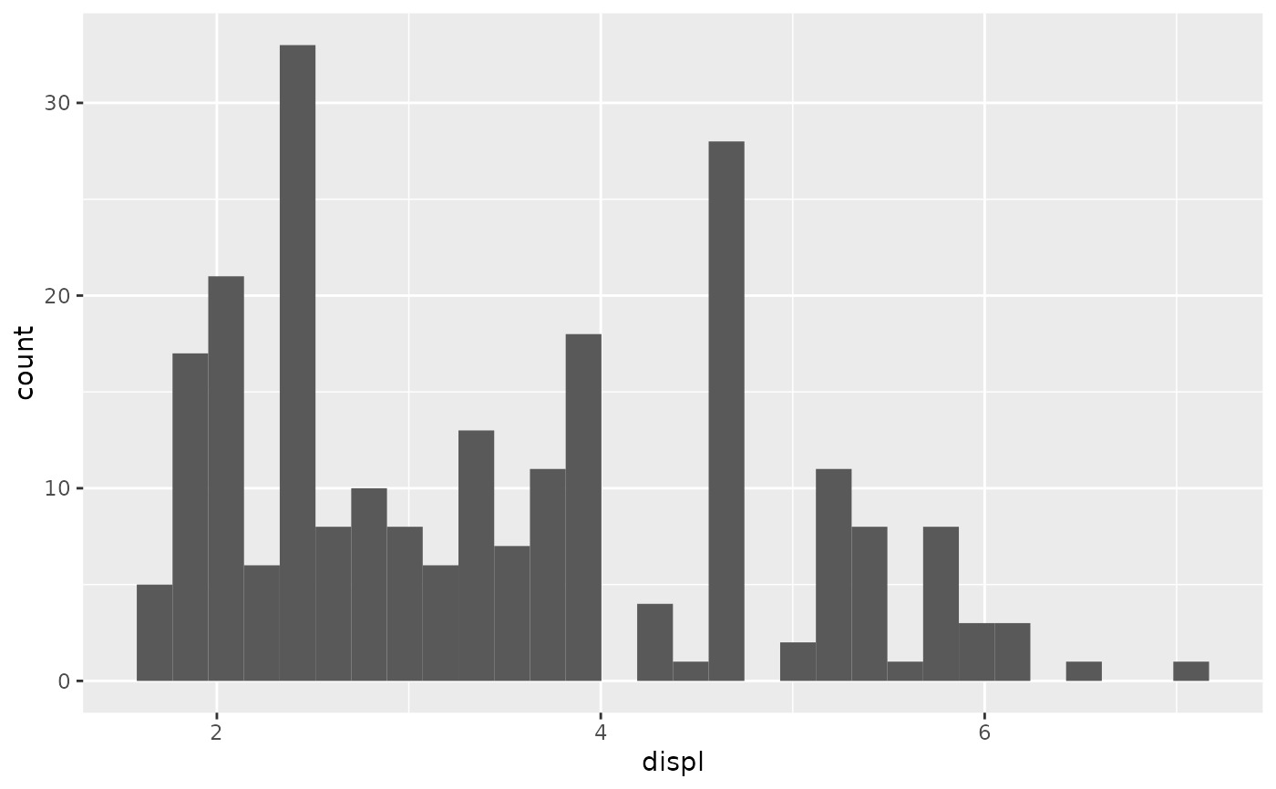
# Default histogram display
ggplot(mpg, aes(displ)) +
geom_histogram(aes(y = after_stat(count)))
#> `stat_bin()` using `bins = 30`. Pick better value with `binwidth`.
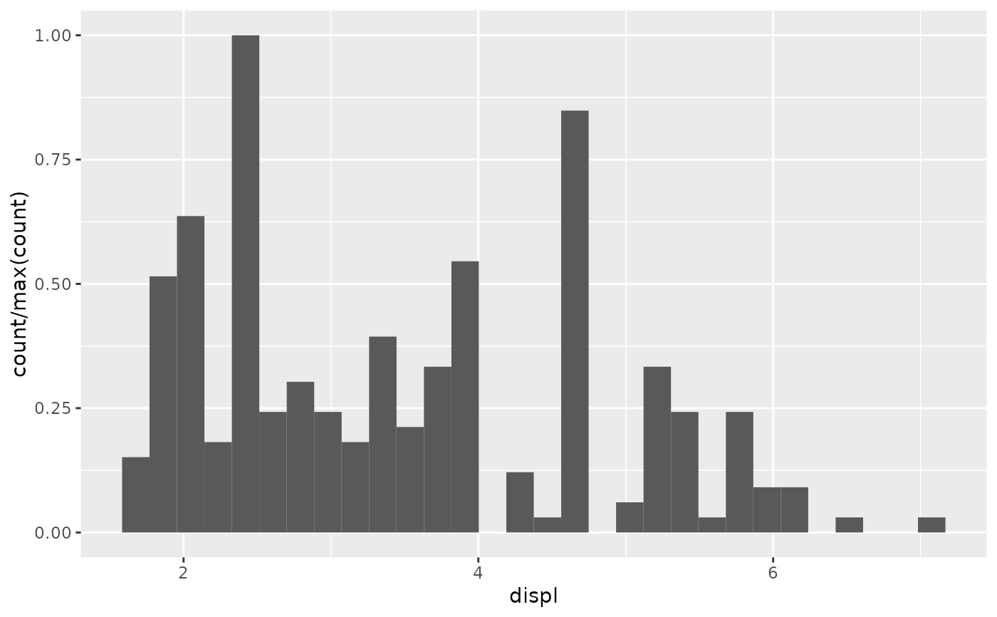
 # Scale tallest bin to 1
ggplot(mpg, aes(displ)) +
geom_histogram(aes(y = after_stat(count / max(count))))
#> `stat_bin()` using `bins = 30`. Pick better value with `binwidth`.
# Scale tallest bin to 1
ggplot(mpg, aes(displ)) +
geom_histogram(aes(y = after_stat(count / max(count))))
#> `stat_bin()` using `bins = 30`. Pick better value with `binwidth`.
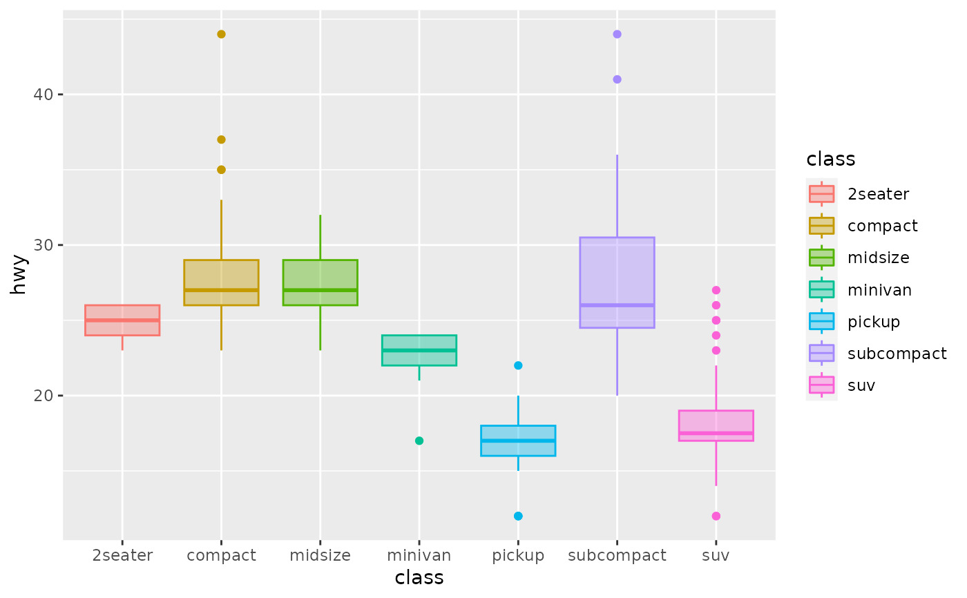
 # Use a transparent version of colour for fill
ggplot(mpg, aes(class, hwy)) +
geom_boxplot(aes(colour = class, fill = after_scale(alpha(colour, 0.4))))
# Use a transparent version of colour for fill
ggplot(mpg, aes(class, hwy)) +
geom_boxplot(aes(colour = class, fill = after_scale(alpha(colour, 0.4))))
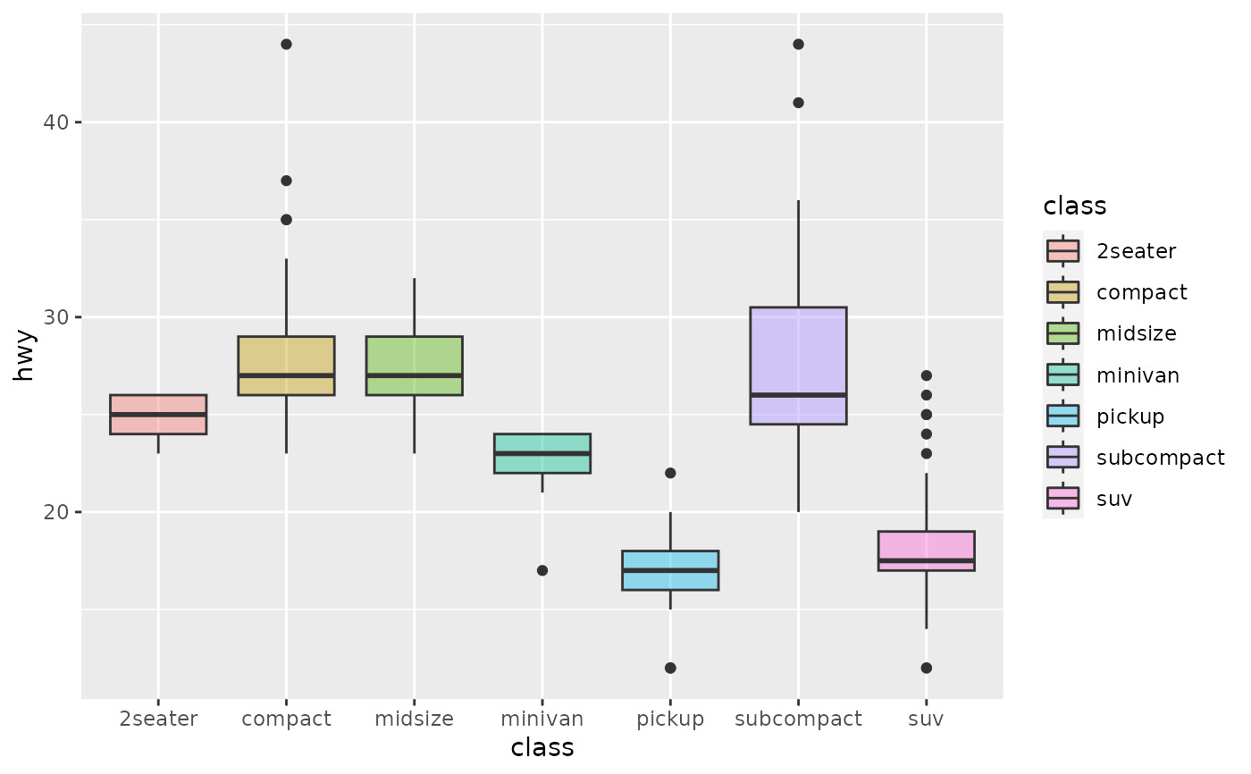
 # Use stage to modify the scaled fill
ggplot(mpg, aes(class, hwy)) +
geom_boxplot(aes(fill = stage(class, after_scale = alpha(fill, 0.4))))
# Use stage to modify the scaled fill
ggplot(mpg, aes(class, hwy)) +
geom_boxplot(aes(fill = stage(class, after_scale = alpha(fill, 0.4))))
 # Making a proportional stacked density plot
ggplot(mpg, aes(cty)) +
geom_density(
aes(
colour = factor(cyl),
fill = after_scale(alpha(colour, 0.3)),
y = after_stat(count / sum(n[!duplicated(group)]))
),
position = "stack", bw = 1
) +
geom_density(bw = 1)
# Making a proportional stacked density plot
ggplot(mpg, aes(cty)) +
geom_density(
aes(
colour = factor(cyl),
fill = after_scale(alpha(colour, 0.3)),
y = after_stat(count / sum(n[!duplicated(group)]))
),
position = "stack", bw = 1
) +
geom_density(bw = 1)
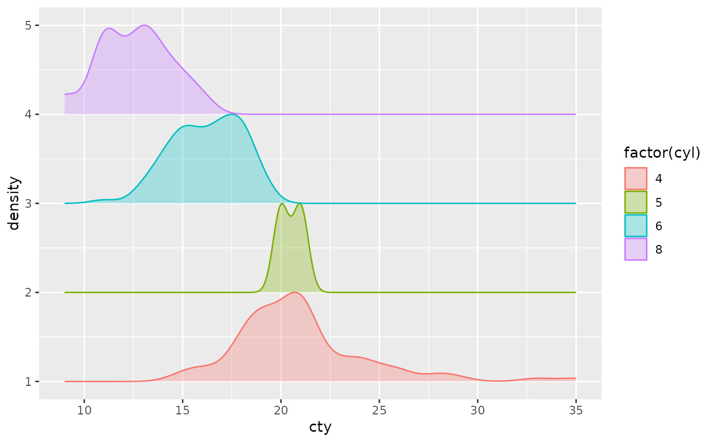
 # Imitating a ridgeline plot
ggplot(mpg, aes(cty, colour = factor(cyl))) +
geom_ribbon(
stat = "density", outline.type = "upper",
aes(
fill = after_scale(alpha(colour, 0.3)),
ymin = after_stat(group),
ymax = after_stat(group + ndensity)
)
)
# Imitating a ridgeline plot
ggplot(mpg, aes(cty, colour = factor(cyl))) +
geom_ribbon(
stat = "density", outline.type = "upper",
aes(
fill = after_scale(alpha(colour, 0.3)),
ymin = after_stat(group),
ymax = after_stat(group + ndensity)
)
)
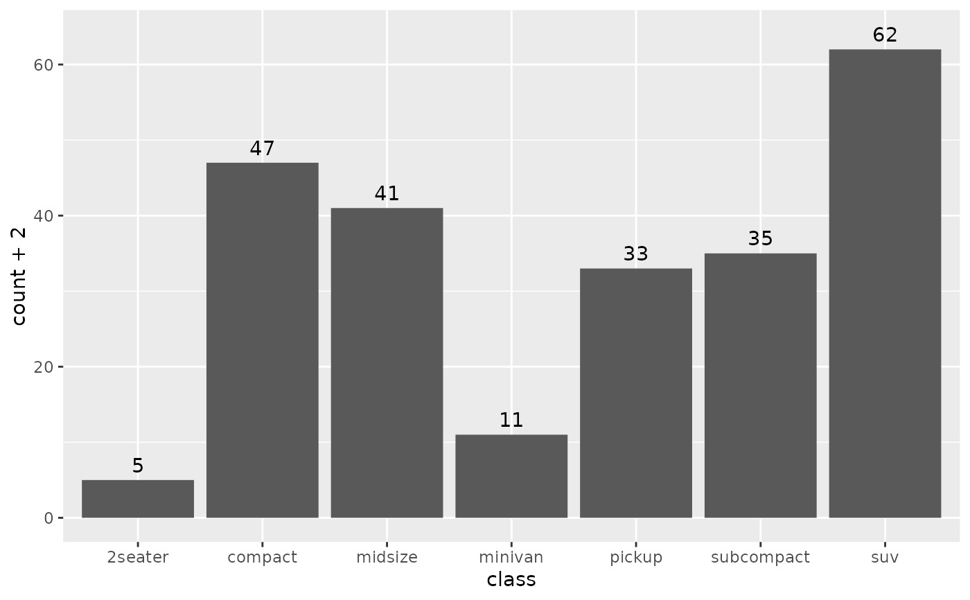
 # Labelling a bar plot
ggplot(mpg, aes(class)) +
geom_bar() +
geom_text(
aes(
y = after_stat(count + 2),
label = after_stat(count)
),
stat = "count"
)
# Labelling a bar plot
ggplot(mpg, aes(class)) +
geom_bar() +
geom_text(
aes(
y = after_stat(count + 2),
label = after_stat(count)
),
stat = "count"
)
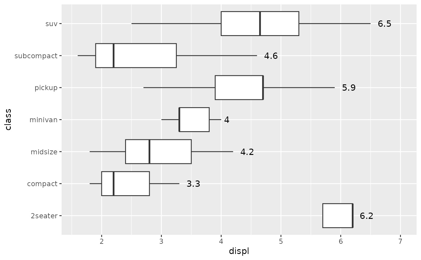
 # Labelling the upper hinge of a boxplot,
# inspired by June Choe
ggplot(mpg, aes(displ, class)) +
geom_boxplot(outlier.shape = NA) +
geom_text(
aes(
label = after_stat(xmax),
x = stage(displ, after_stat = xmax)
),
stat = "boxplot", hjust = -0.5
)
# Labelling the upper hinge of a boxplot,
# inspired by June Choe
ggplot(mpg, aes(displ, class)) +
geom_boxplot(outlier.shape = NA) +
geom_text(
aes(
label = after_stat(xmax),
x = stage(displ, after_stat = xmax)
),
stat = "boxplot", hjust = -0.5
)
相关用法
- R ggplot2 aes 构建美学映射
- R ggplot2 annotation_logticks 注释:记录刻度线
- R ggplot2 annotation_custom 注释:自定义grob
- R ggplot2 annotate 创建注释层
- R ggplot2 annotation_map 注释:Map
- R ggplot2 annotation_raster 注释:高性能矩形平铺
- R ggplot2 as_labeller 强制贴标机函数
- R ggplot2 vars 引用分面变量
- R ggplot2 position_stack 将重叠的对象堆叠在一起
- R ggplot2 geom_qq 分位数-分位数图
- R ggplot2 geom_spoke 由位置、方向和距离参数化的线段
- R ggplot2 geom_quantile 分位数回归
- R ggplot2 geom_text 文本
- R ggplot2 get_alt_text 从绘图中提取替代文本
- R ggplot2 geom_ribbon 函数区和面积图
- R ggplot2 stat_ellipse 计算法行数据椭圆
- R ggplot2 resolution 计算数值向量的“分辨率”
- R ggplot2 geom_boxplot 盒须图(Tukey 风格)
- R ggplot2 lims 设置规模限制
- R ggplot2 geom_hex 二维箱计数的六边形热图
- R ggplot2 scale_gradient 渐变色阶
- R ggplot2 scale_shape 形状比例,又称字形
- R ggplot2 geom_bar 条形图
- R ggplot2 draw_key 图例的关键字形
- R ggplot2 label_bquote 带有数学表达式的标签
注:本文由纯净天空筛选整理自Hadley Wickham等大神的英文原创作品 Control aesthetic evaluation。非经特殊声明,原始代码版权归原作者所有,本译文未经允许或授权,请勿转载或复制。