計算並繪製核密度估計,它是直方圖的平滑版本。對於來自底層平滑分布的連續數據,這是直方圖的有用替代方案。
用法
geom_density(
  mapping = NULL,
  data = NULL,
  stat = "density",
  position = "identity",
  ...,
  na.rm = FALSE,
  orientation = NA,
  show.legend = NA,
  inherit.aes = TRUE,
  outline.type = "upper"
)

stat_density(
  mapping = NULL,
  data = NULL,
  geom = "area",
  position = "stack",
  ...,
  bw = "nrd0",
  adjust = 1,
  kernel = "gaussian",
  n = 512,
  trim = FALSE,
  na.rm = FALSE,
  bounds = c(-Inf, Inf),
  orientation = NA,
  show.legend = NA,
  inherit.aes = TRUE
)
參數
- mapping
-
由
aes()創建的一組美學映射。如果指定且inherit.aes = TRUE(默認),它將與繪圖頂層的默認映射組合。如果沒有繪圖映射,則必須提供mapping。 - data
-
該層要顯示的數據。有以下三種選擇:
如果默認為
NULL,則數據繼承自ggplot()調用中指定的繪圖數據。data.frame或其他對象將覆蓋繪圖數據。所有對象都將被強化以生成 DataFrame 。請參閱fortify()將為其創建變量。將使用單個參數(繪圖數據)調用
function。返回值必須是data.frame,並將用作圖層數據。可以從formula創建function(例如~ head(.x, 10))。 - position
-
位置調整,可以是命名調整的字符串(例如
"jitter"使用position_jitter),也可以是調用位置調整函數的結果。如果需要更改調整設置,請使用後者。 - ...
-
其他參數傳遞給
layer()。這些通常是美學,用於將美學設置為固定值,例如colour = "red"或size = 3。它們也可能是配對的 geom/stat 的參數。 - na.rm
-
如果
FALSE,則默認缺失值將被刪除並帶有警告。如果TRUE,缺失值將被靜默刪除。 - orientation
-
層的方向。默認值 (
NA) 自動根據美學映射確定方向。萬一失敗,可以通過將orientation設置為"x"或"y"來顯式給出。有關更多詳細信息,請參閱方向部分。 - show.legend
-
合乎邏輯的。該層是否應該包含在圖例中?
NA(默認值)包括是否映射了任何美學。FALSE從不包含,而TRUE始終包含。它也可以是一個命名的邏輯向量,以精細地選擇要顯示的美學。 - inherit.aes
-
如果
FALSE,則覆蓋默認美學,而不是與它們組合。這對於定義數據和美觀的輔助函數最有用,並且不應繼承默認繪圖規範的行為,例如borders()。 - outline.type
-
區域輪廓的類型;
"both"繪製上下兩條線,"upper"/"lower"僅繪製相應的線。"full"在該區域周圍繪製一個閉合多邊形。 - geom, stat
-
用於覆蓋
geom_density()和stat_density()之間的默認連接。 - bw
-
要使用的平滑帶寬。如果是數字,則為平滑內核的標準差。如果是字符,則選擇帶寬的規則,如
stats::bw.nrd()中列出。 - adjust
-
多重帶寬調整。這使得在仍然使用帶寬估計器的同時調整帶寬成為可能。例如
adjust = 1/2表示使用默認帶寬的一半。 - kernel
-
核心。請參閱
density()中的可用內核列表。 - n
-
要估計密度的等距點的數量,應該是 2 的冪,有關詳細信息,請參閱
density() - trim
-
如果是
FALSE(默認值),則每個密度都是在數據的整個範圍內計算的。如果是TRUE,則每個密度都是在該組的範圍內計算的:這通常意味著估計的 x 值不會line-up,因此您將無法堆疊密度值。僅當您在一張圖中顯示多個密度或手動調整比例限製時,此參數才有意義。 - bounds
-
已知估計數據的下限和上限。默認
c(-Inf, Inf)意味著沒有(有限)邊界。如果任何邊界是有限的,則默認密度估計的邊界效應將通過在最近邊周圍反射bounds之外的尾部來糾正。超出範圍的數據點將被刪除並發出警告。
方向
該幾何體以不同的方式對待每個軸,因此可以有兩個方向。通常,方向很容易從給定映射和使用的位置比例類型的組合中推斷出來。因此,ggplot2 默認情況下會嘗試猜測圖層應具有哪個方向。在極少數情況下,方向不明確,猜測可能會失敗。在這種情況下,可以直接使用 orientation 參數指定方向,該參數可以是 "x" 或 "y" 。該值給出了幾何圖形應沿著的軸,"x" 是您期望的幾何圖形的默認方向。
美學
geom_density() 理解以下美學(所需的美學以粗體顯示):
-
x -
y -
alpha -
colour -
fill -
group -
linetype -
linewidth -
weight
在 vignette("ggplot2-specs") 中了解有關設置這些美學的更多信息。
計算變量
這些是由層的 'stat' 部分計算的,可以使用 delayed evaluation 訪問。
-
after_stat(density)
密度估計。 -
after_stat(count)
密度 * 點數 - 對於堆積密度圖很有用。 -
after_stat(scaled)
密度估計,縮放至最大值 1。 -
after_stat(n)
點數。 -
after_stat(ndensity)
別名為scaled,鏡像語法stat_bin().
也可以看看
有關顯示連續分布的其他方法,請參閱geom_histogram()、geom_freqpoly()。有關緊湊密度顯示,請參閱geom_violin()。
例子
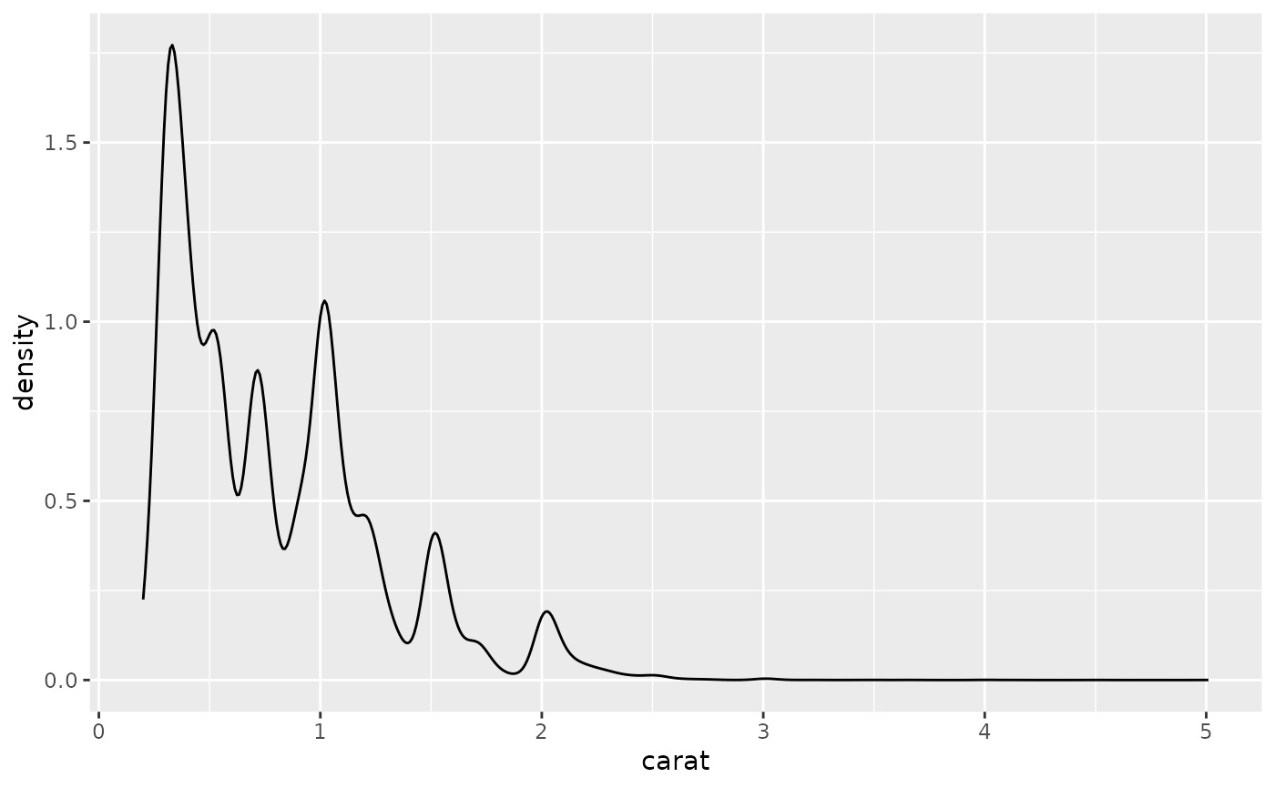
ggplot(diamonds, aes(carat)) +
geom_density()
 # Map the values to y to flip the orientation
ggplot(diamonds, aes(y = carat)) +
geom_density()
# Map the values to y to flip the orientation
ggplot(diamonds, aes(y = carat)) +
geom_density()
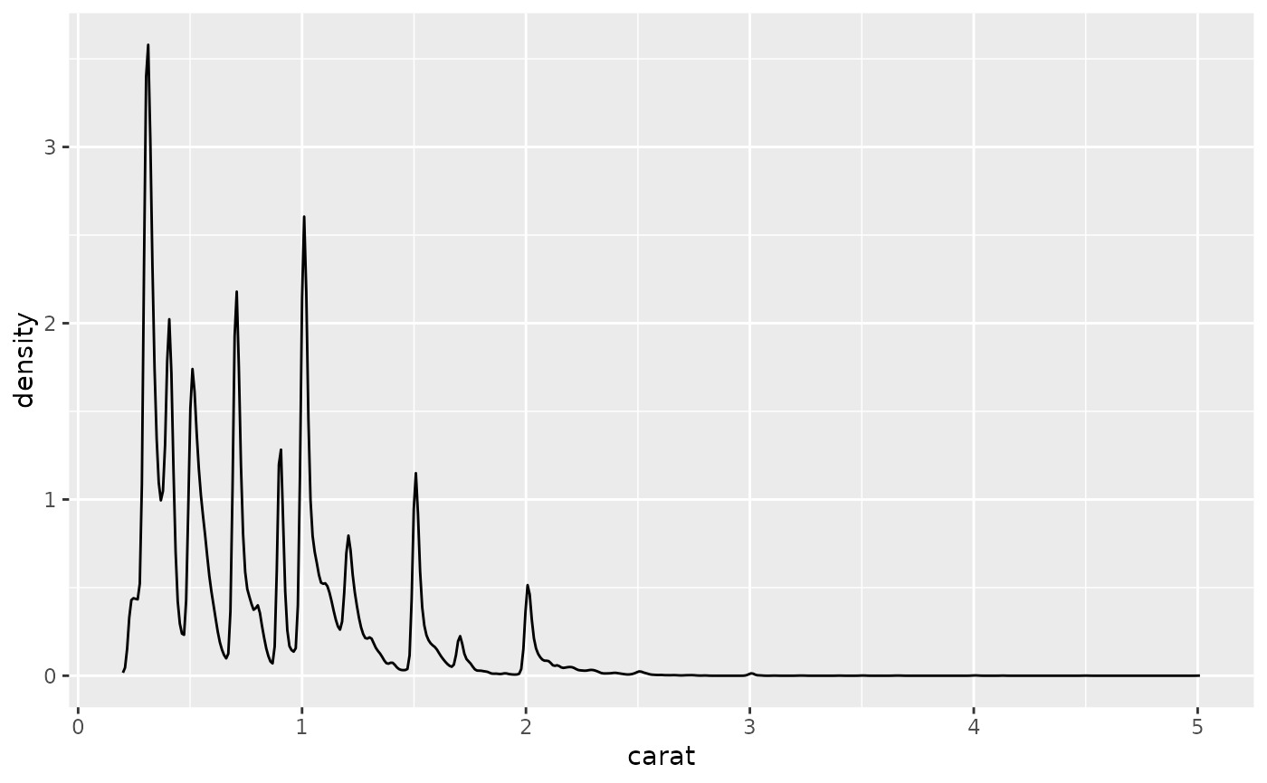
 ggplot(diamonds, aes(carat)) +
geom_density(adjust = 1/5)
ggplot(diamonds, aes(carat)) +
geom_density(adjust = 1/5)
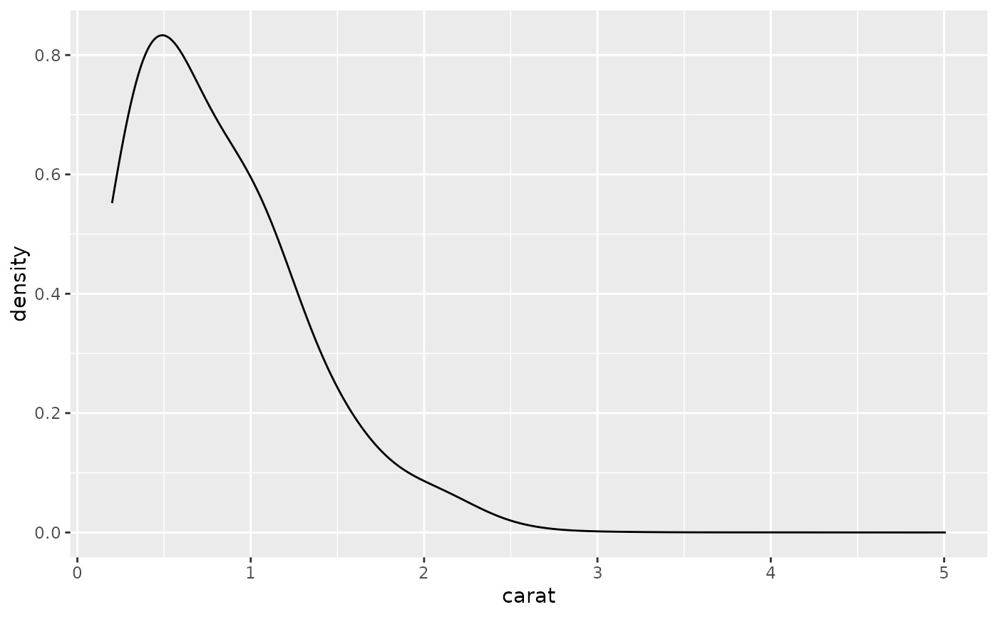
 ggplot(diamonds, aes(carat)) +
geom_density(adjust = 5)
ggplot(diamonds, aes(carat)) +
geom_density(adjust = 5)
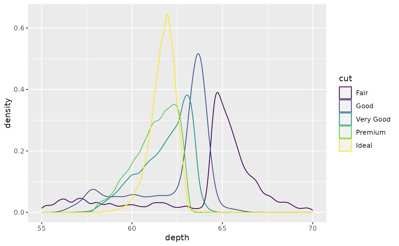
 ggplot(diamonds, aes(depth, colour = cut)) +
geom_density() +
xlim(55, 70)
#> Warning: Removed 45 rows containing non-finite values (`stat_density()`).
ggplot(diamonds, aes(depth, colour = cut)) +
geom_density() +
xlim(55, 70)
#> Warning: Removed 45 rows containing non-finite values (`stat_density()`).
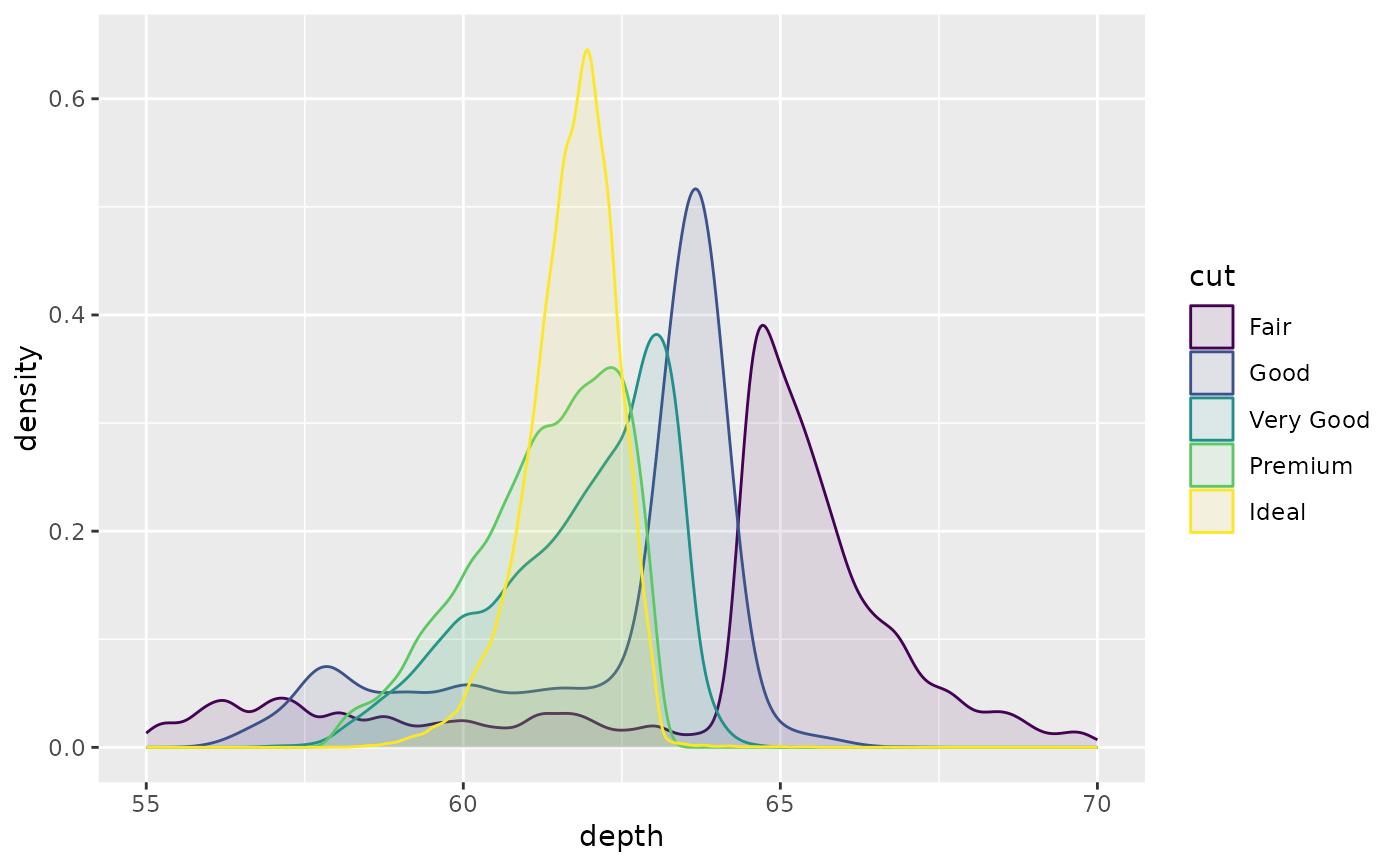
 ggplot(diamonds, aes(depth, fill = cut, colour = cut)) +
geom_density(alpha = 0.1) +
xlim(55, 70)
#> Warning: Removed 45 rows containing non-finite values (`stat_density()`).
ggplot(diamonds, aes(depth, fill = cut, colour = cut)) +
geom_density(alpha = 0.1) +
xlim(55, 70)
#> Warning: Removed 45 rows containing non-finite values (`stat_density()`).
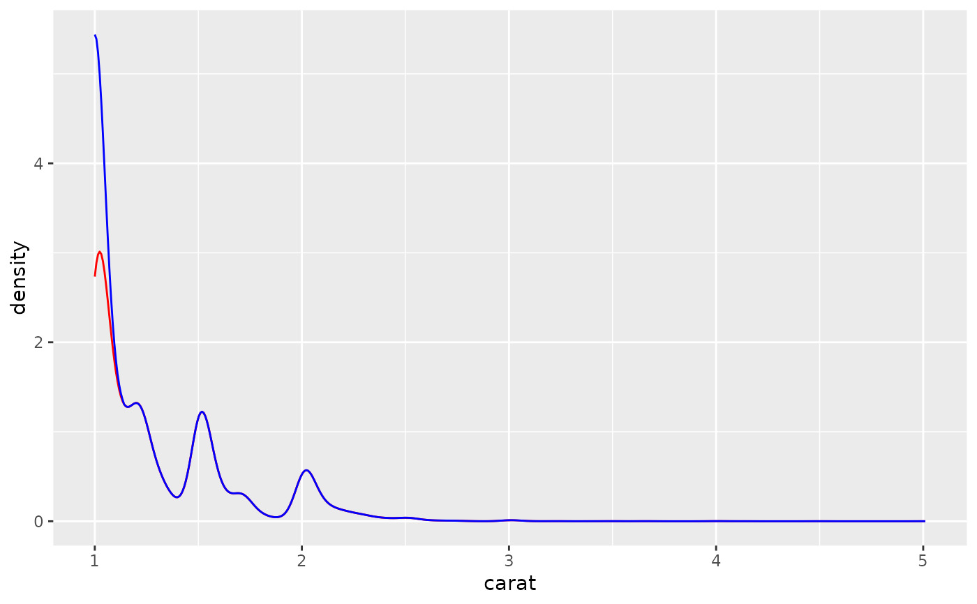
 # Use `bounds` to adjust computation for known data limits
big_diamonds <- diamonds[diamonds$carat >= 1, ]
ggplot(big_diamonds, aes(carat)) +
geom_density(color = 'red') +
geom_density(bounds = c(1, Inf), color = 'blue')
# Use `bounds` to adjust computation for known data limits
big_diamonds <- diamonds[diamonds$carat >= 1, ]
ggplot(big_diamonds, aes(carat)) +
geom_density(color = 'red') +
geom_density(bounds = c(1, Inf), color = 'blue')
 # \donttest{
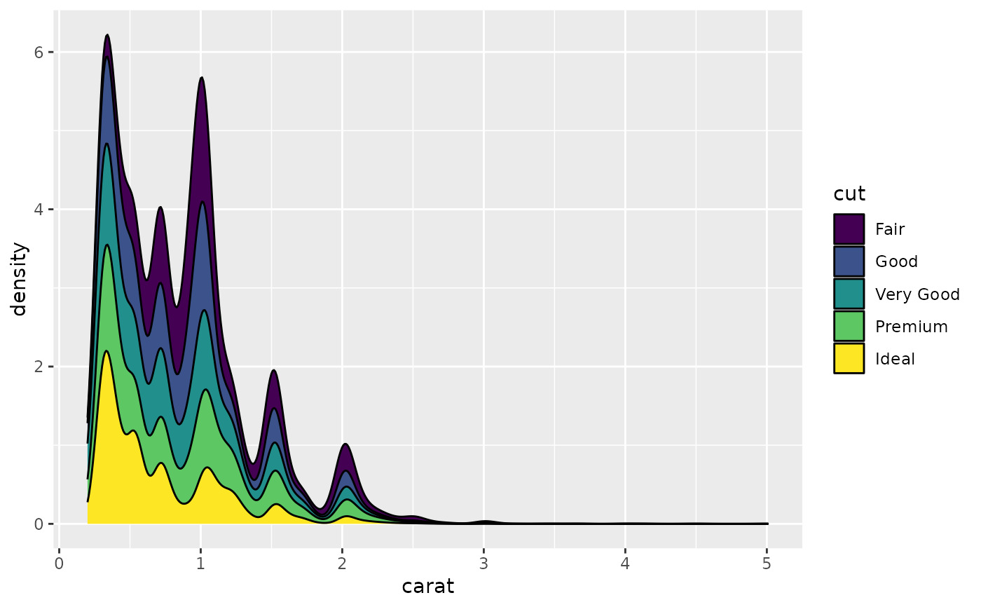
# Stacked density plots: if you want to create a stacked density plot, you
# probably want to 'count' (density * n) variable instead of the default
# density
# Loses marginal densities
ggplot(diamonds, aes(carat, fill = cut)) +
geom_density(position = "stack")
# \donttest{
# Stacked density plots: if you want to create a stacked density plot, you
# probably want to 'count' (density * n) variable instead of the default
# density
# Loses marginal densities
ggplot(diamonds, aes(carat, fill = cut)) +
geom_density(position = "stack")
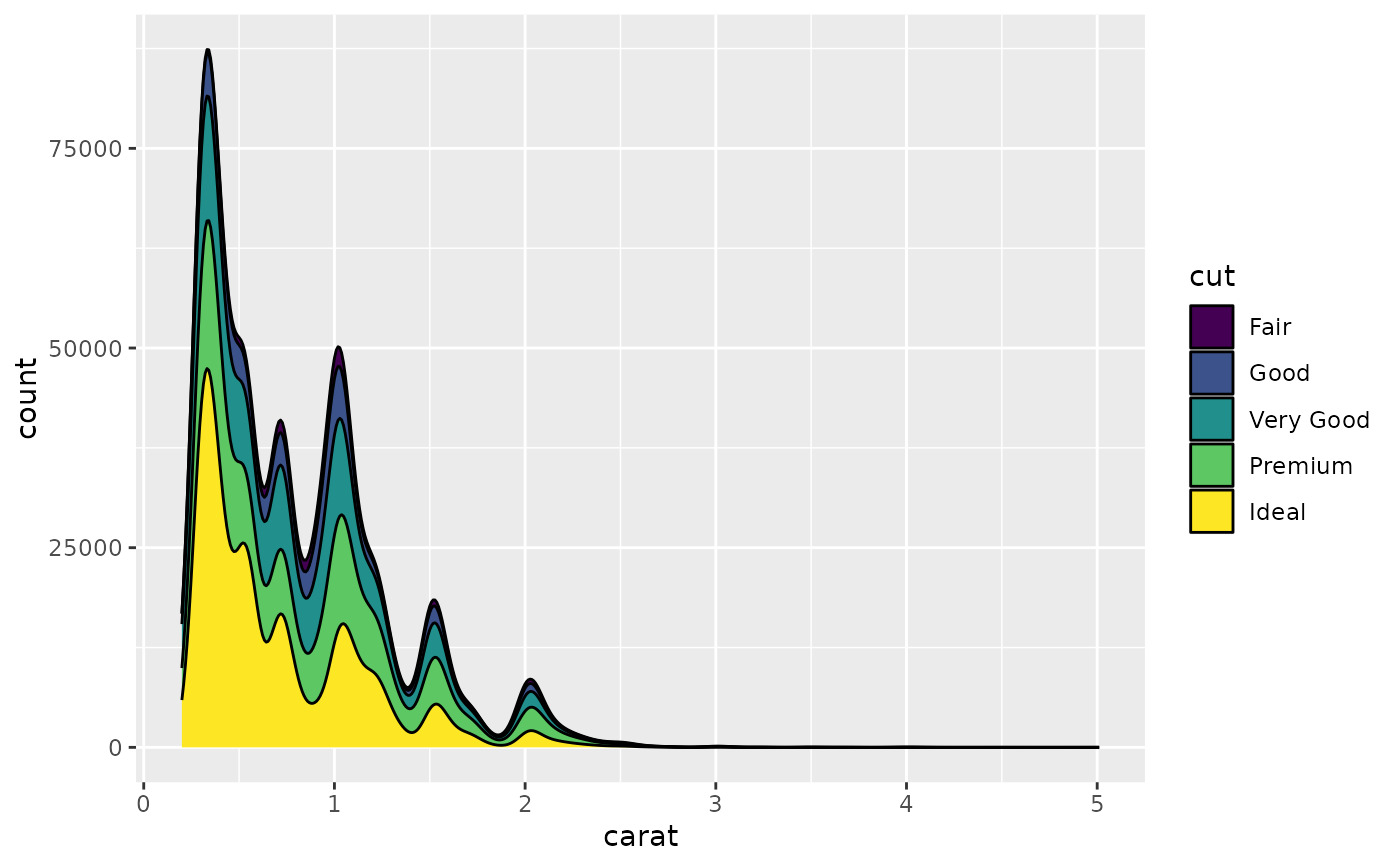
 # Preserves marginal densities
ggplot(diamonds, aes(carat, after_stat(count), fill = cut)) +
geom_density(position = "stack")
# Preserves marginal densities
ggplot(diamonds, aes(carat, after_stat(count), fill = cut)) +
geom_density(position = "stack")
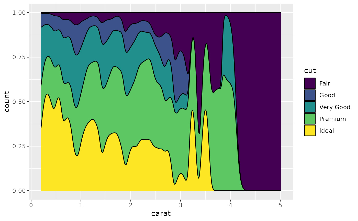
 # You can use position="fill" to produce a conditional density estimate
ggplot(diamonds, aes(carat, after_stat(count), fill = cut)) +
geom_density(position = "fill")
# You can use position="fill" to produce a conditional density estimate
ggplot(diamonds, aes(carat, after_stat(count), fill = cut)) +
geom_density(position = "fill")
 # }
# }
相關用法
- R ggplot2 geom_density_2d 二維密度估計的等值線
- R ggplot2 geom_dotplot 點圖
- R ggplot2 geom_qq 分位數-分位數圖
- R ggplot2 geom_spoke 由位置、方向和距離參數化的線段
- R ggplot2 geom_quantile 分位數回歸
- R ggplot2 geom_text 文本
- R ggplot2 geom_ribbon 函數區和麵積圖
- R ggplot2 geom_boxplot 盒須圖(Tukey 風格)
- R ggplot2 geom_hex 二維箱計數的六邊形熱圖
- R ggplot2 geom_bar 條形圖
- R ggplot2 geom_bin_2d 二維 bin 計數熱圖
- R ggplot2 geom_jitter 抖動點
- R ggplot2 geom_point 積分
- R ggplot2 geom_linerange 垂直間隔:線、橫線和誤差線
- R ggplot2 geom_blank 什麽也不畫
- R ggplot2 geom_path 連接觀察結果
- R ggplot2 geom_violin 小提琴情節
- R ggplot2 geom_errorbarh 水平誤差線
- R ggplot2 geom_function 將函數繪製為連續曲線
- R ggplot2 geom_polygon 多邊形
- R ggplot2 geom_histogram 直方圖和頻數多邊形
- R ggplot2 geom_tile 矩形
- R ggplot2 geom_segment 線段和曲線
- R ggplot2 geom_map 參考Map中的多邊形
- R ggplot2 geom_abline 參考線:水平、垂直和對角線
注:本文由純淨天空篩選整理自Hadley Wickham等大神的英文原創作品 Smoothed density estimates。非經特殊聲明,原始代碼版權歸原作者所有,本譯文未經允許或授權,請勿轉載或複製。