这是一个变体 geom_point(),它计算每个位置的观测数量,然后将计数映射到点区域。当您有离散数据和过度绘制时,它很有用。
用法
geom_count(
  mapping = NULL,
  data = NULL,
  stat = "sum",
  position = "identity",
  ...,
  na.rm = FALSE,
  show.legend = NA,
  inherit.aes = TRUE
)

stat_sum(
  mapping = NULL,
  data = NULL,
  geom = "point",
  position = "identity",
  ...,
  na.rm = FALSE,
  show.legend = NA,
  inherit.aes = TRUE
)
参数
- mapping
-
由
aes()创建的一组美学映射。如果指定且inherit.aes = TRUE(默认),它将与绘图顶层的默认映射组合。如果没有绘图映射,则必须提供mapping。 - data
-
该层要显示的数据。有以下三种选择:
如果默认为
NULL,则数据继承自ggplot()调用中指定的绘图数据。data.frame或其他对象将覆盖绘图数据。所有对象都将被强化以生成 DataFrame 。请参阅fortify()将为其创建变量。将使用单个参数(绘图数据)调用
function。返回值必须是data.frame,并将用作图层数据。可以从formula创建function(例如~ head(.x, 10))。 - position
-
位置调整,可以是命名调整的字符串(例如
"jitter"使用position_jitter),也可以是调用位置调整函数的结果。如果需要更改调整设置,请使用后者。 - ...
-
其他参数传递给
layer()。这些通常是美学,用于将美学设置为固定值,例如colour = "red"或size = 3。它们也可能是配对的 geom/stat 的参数。 - na.rm
-
如果
FALSE,则默认缺失值将被删除并带有警告。如果TRUE,缺失值将被静默删除。 - show.legend
-
合乎逻辑的。该层是否应该包含在图例中?
NA(默认值)包括是否映射了任何美学。FALSE从不包含,而TRUE始终包含。它也可以是一个命名的逻辑向量,以精细地选择要显示的美学。 - inherit.aes
-
如果
FALSE,则覆盖默认美学,而不是与它们组合。这对于定义数据和美观的辅助函数最有用,并且不应继承默认绘图规范的行为,例如borders()。 - geom, stat
-
用于覆盖
geom_count()和stat_sum()之间的默认连接。
美学
geom_point() 理解以下美学(所需的美学以粗体显示):
-
x -
y -
alpha -
colour -
fill -
group -
shape -
size -
stroke
在 vignette("ggplot2-specs") 中了解有关设置这些美学的更多信息。
计算变量
这些是由层的 'stat' 部分计算的,可以使用 delayed evaluation 访问。
-
after_stat(n)
位置观测值的数量。 -
after_stat(prop)
该面板中该位置的点的百分比。
也可以看看
对于连续的 x 和 y ,请使用 geom_bin2d() 。
例子
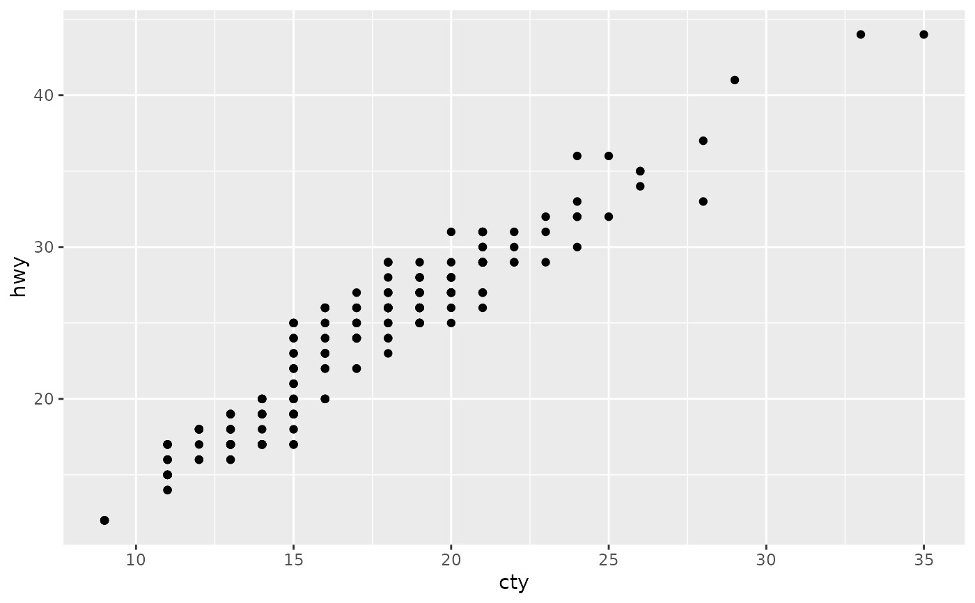
ggplot(mpg, aes(cty, hwy)) +
geom_point()
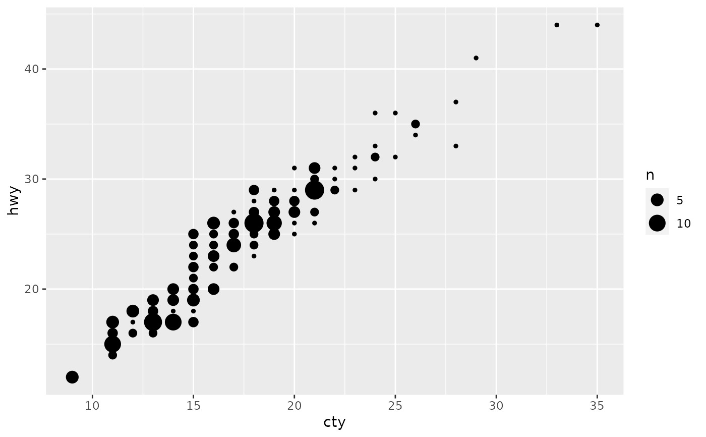
 ggplot(mpg, aes(cty, hwy)) +
geom_count()
ggplot(mpg, aes(cty, hwy)) +
geom_count()
 # Best used in conjunction with scale_size_area which ensures that
# counts of zero would be given size 0. Doesn't make much different
# here because the smallest count is already close to 0.
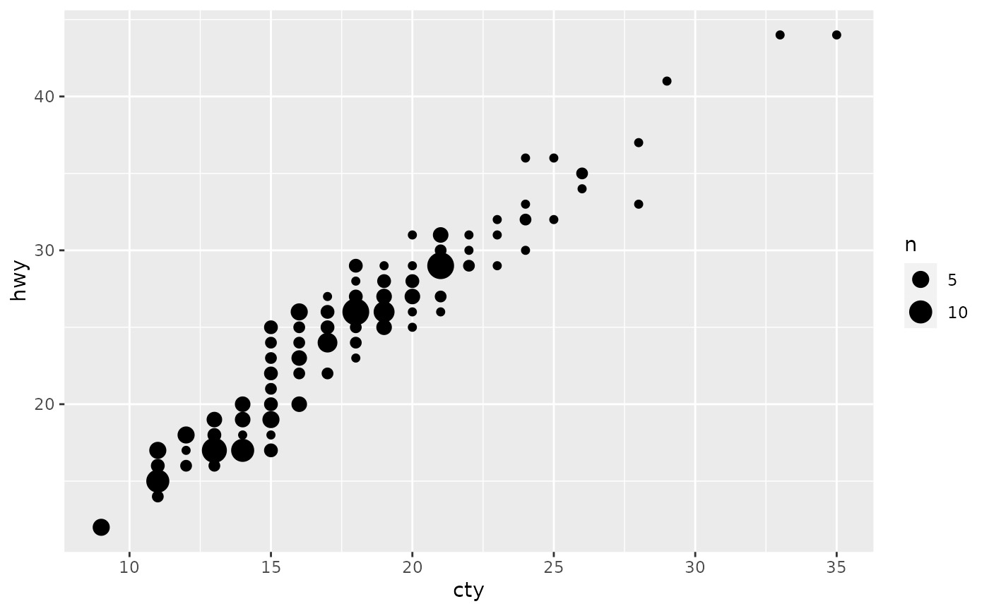
ggplot(mpg, aes(cty, hwy)) +
geom_count() +
scale_size_area()
# Best used in conjunction with scale_size_area which ensures that
# counts of zero would be given size 0. Doesn't make much different
# here because the smallest count is already close to 0.
ggplot(mpg, aes(cty, hwy)) +
geom_count() +
scale_size_area()
 # Display proportions instead of counts -------------------------------------
# By default, all categorical variables in the plot form the groups.
# Specifying geom_count without a group identifier leads to a plot which is
# not useful:
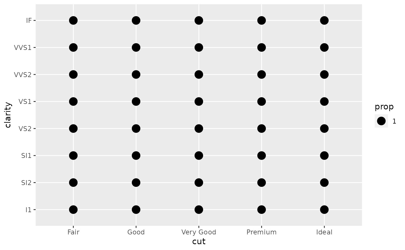
d <- ggplot(diamonds, aes(x = cut, y = clarity))
d + geom_count(aes(size = after_stat(prop)))
# Display proportions instead of counts -------------------------------------
# By default, all categorical variables in the plot form the groups.
# Specifying geom_count without a group identifier leads to a plot which is
# not useful:
d <- ggplot(diamonds, aes(x = cut, y = clarity))
d + geom_count(aes(size = after_stat(prop)))
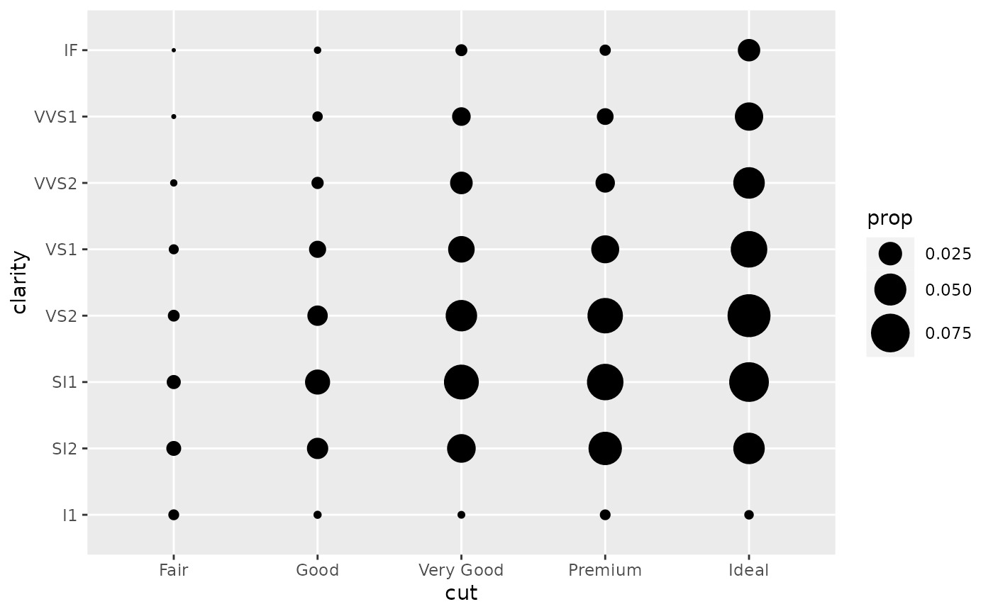
 # To correct this problem and achieve a more desirable plot, we need
# to specify which group the proportion is to be calculated over.
d + geom_count(aes(size = after_stat(prop), group = 1)) +
scale_size_area(max_size = 10)
# To correct this problem and achieve a more desirable plot, we need
# to specify which group the proportion is to be calculated over.
d + geom_count(aes(size = after_stat(prop), group = 1)) +
scale_size_area(max_size = 10)
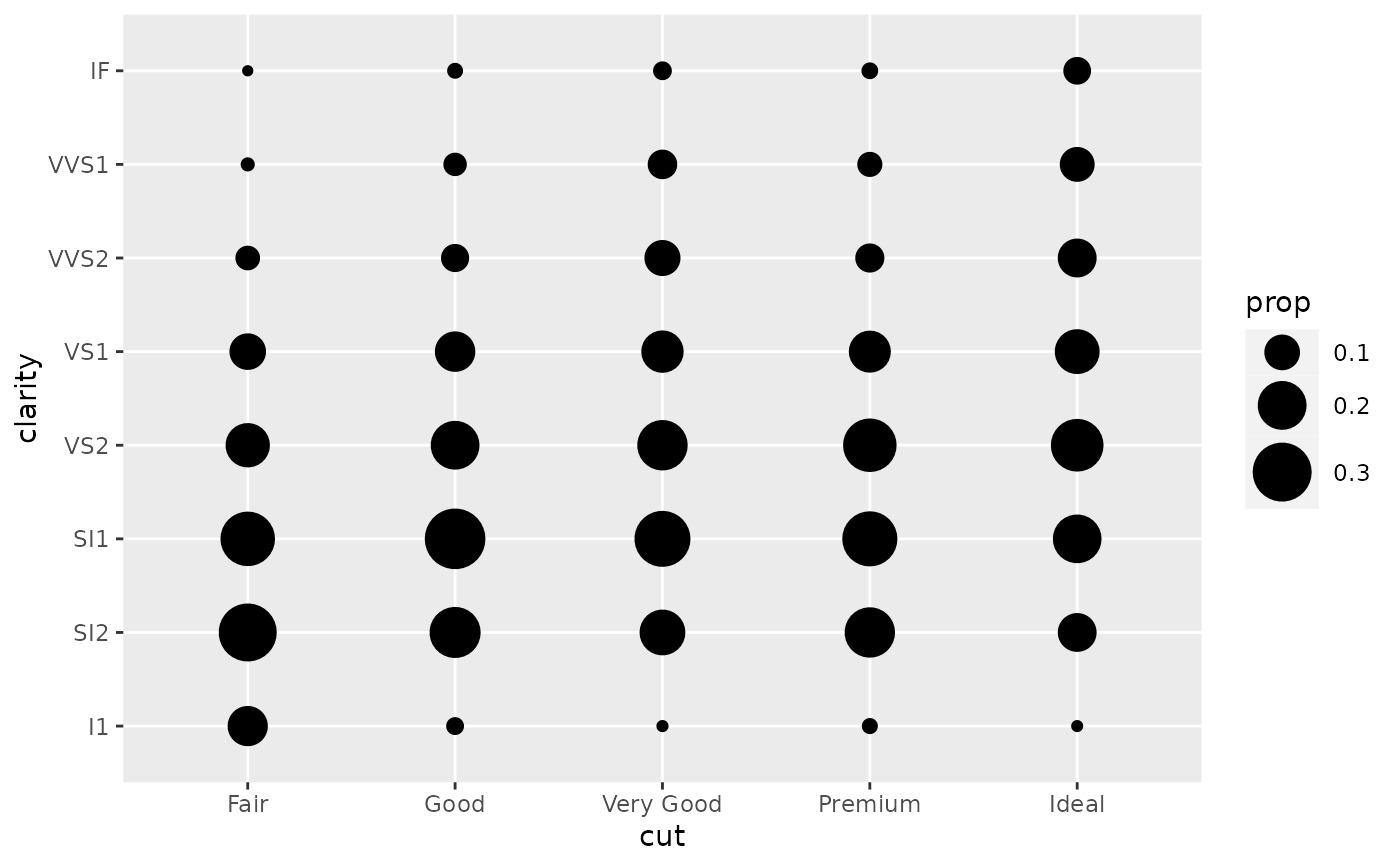
 # Or group by x/y variables to have rows/columns sum to 1.
d + geom_count(aes(size = after_stat(prop), group = cut)) +
scale_size_area(max_size = 10)
# Or group by x/y variables to have rows/columns sum to 1.
d + geom_count(aes(size = after_stat(prop), group = cut)) +
scale_size_area(max_size = 10)
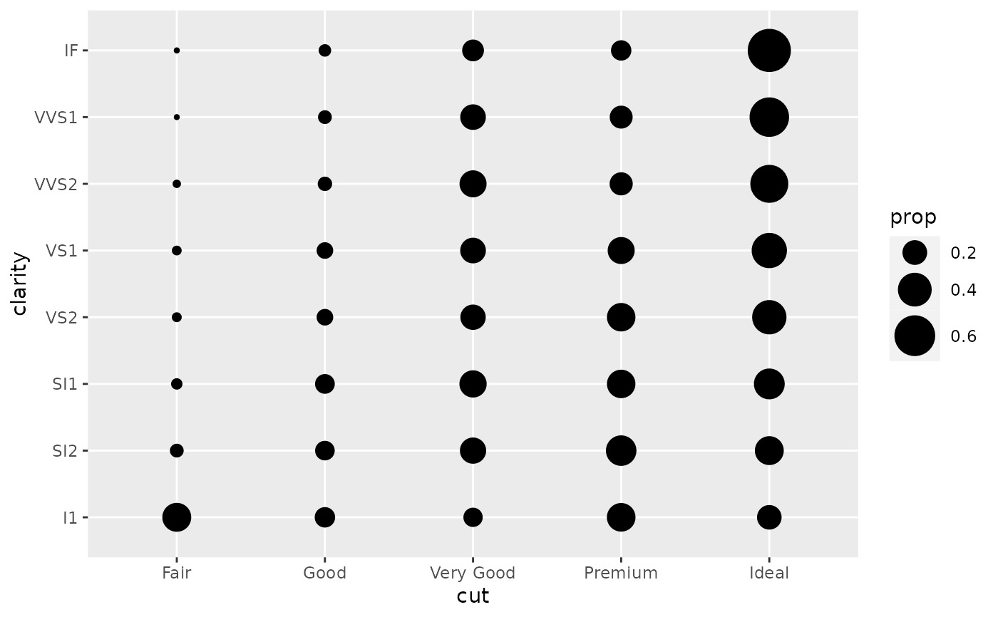
 d + geom_count(aes(size = after_stat(prop), group = clarity)) +
scale_size_area(max_size = 10)
d + geom_count(aes(size = after_stat(prop), group = clarity)) +
scale_size_area(max_size = 10)
相关用法
- R ggplot2 geom_contour 3D 表面的 2D 轮廓
- R ggplot2 geom_qq 分位数-分位数图
- R ggplot2 geom_spoke 由位置、方向和距离参数化的线段
- R ggplot2 geom_quantile 分位数回归
- R ggplot2 geom_text 文本
- R ggplot2 geom_ribbon 函数区和面积图
- R ggplot2 geom_boxplot 盒须图(Tukey 风格)
- R ggplot2 geom_hex 二维箱计数的六边形热图
- R ggplot2 geom_bar 条形图
- R ggplot2 geom_bin_2d 二维 bin 计数热图
- R ggplot2 geom_jitter 抖动点
- R ggplot2 geom_point 积分
- R ggplot2 geom_linerange 垂直间隔:线、横线和误差线
- R ggplot2 geom_blank 什么也不画
- R ggplot2 geom_path 连接观察结果
- R ggplot2 geom_violin 小提琴情节
- R ggplot2 geom_dotplot 点图
- R ggplot2 geom_errorbarh 水平误差线
- R ggplot2 geom_function 将函数绘制为连续曲线
- R ggplot2 geom_polygon 多边形
- R ggplot2 geom_histogram 直方图和频数多边形
- R ggplot2 geom_tile 矩形
- R ggplot2 geom_segment 线段和曲线
- R ggplot2 geom_density_2d 二维密度估计的等值线
- R ggplot2 geom_map 参考Map中的多边形
注:本文由纯净天空筛选整理自Hadley Wickham等大神的英文原创作品 Count overlapping points。非经特殊声明,原始代码版权归原作者所有,本译文未经允许或授权,请勿转载或复制。