Python SciPy special.y0_zeros用法及代码示例

本文简要介绍 python 语言中 scipy.special.y0_zeros 的用法。

用法:

scipy.special.y0_zeros(nt, complex=False)#

计算贝塞尔函数 Y0(z) 的 nt 个零点，以及每个零点处的导数。

每个零 z0 处的导数由 Y0’(z0) = -Y1(z0) 给出。

参数 ：：

nt： int

要返回的零数

complex： 布尔值，默认为 False

设置为 False 仅返回实数零；设置为 True 仅返回具有负实部和正虚部的复数零。请注意，后者的复共轭也是函数的零，但此例程不返回。

返回 ：：

z0n： ndarray

Y0(z)的第n个零的位置

y0pz0n： ndarray

第 n 个零的导数 Y0’(z0) 值

参考：

[1]

张善杰和金建明。 “特殊函数的计算”，John Wiley and Sons，1996 年，第 5 章。https://people.sc.fsu.edu/~jburkardt/f77_src/special_functions/special_functions.html

例子：

计算 \(Y_0\) 的前 4 个实根和根处的导数：

>>> import numpy as np
>>> from scipy.special import y0_zeros
>>> zeros, grads = y0_zeros(4)
>>> with np.printoptions(precision=5):
...     print(f"Roots: {zeros}")
...     print(f"Gradients: {grads}")
Roots: [ 0.89358+0.j  3.95768+0.j  7.08605+0.j 10.22235+0.j]
Gradients: [-0.87942+0.j  0.40254+0.j -0.3001 +0.j  0.2497 +0.j]

绘制 \(Y_0\) 的实部和前四个计算根。

>>> import matplotlib.pyplot as plt
>>> from scipy.special import y0
>>> xmin = 0
>>> xmax = 11
>>> x = np.linspace(xmin, xmax, 500)
>>> fig, ax = plt.subplots()
>>> ax.hlines(0, xmin, xmax, color='k')
>>> ax.plot(x, y0(x), label=r'$Y_0$')
>>> zeros, grads = y0_zeros(4)
>>> ax.scatter(zeros.real, np.zeros((4, )), s=30, c='r',
...            label=r'$Y_0$_zeros', zorder=5)
>>> ax.set_ylim(-0.5, 0.6)
>>> ax.set_xlim(xmin, xmax)
>>> plt.legend(ncol=2)
>>> plt.show()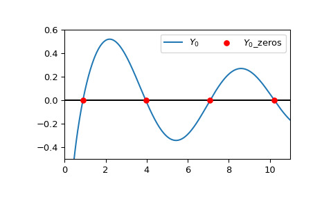

通过设置 complex=True 计算 \(Y_0\) 的前 4 个复数根和根处的导数：

>>> y0_zeros(4, True)
(array([ -2.40301663+0.53988231j,  -5.5198767 +0.54718001j,
         -8.6536724 +0.54841207j, -11.79151203+0.54881912j]),
 array([ 0.10074769-0.88196771j, -0.02924642+0.5871695j ,
         0.01490806-0.46945875j, -0.00937368+0.40230454j]))