Python SciPy special.y1_zeros用法及代码示例

本文简要介绍 python 语言中 scipy.special.y1_zeros 的用法。

用法:

scipy.special.y1_zeros(nt, complex=False)#

计算贝塞尔函数 Y1(z) 的 nt 个零点，以及每个零点处的导数。

每个零 z1 处的导数由 Y1’(z1) = Y0(z1) 给出。

参数 ：：

nt： int

要返回的零数

complex： 布尔值，默认为 False

设置为 False 仅返回实数零；设置为 True 仅返回具有负实部和正虚部的复数零。请注意，后者的复共轭也是函数的零，但此例程不返回。

返回 ：：

z1n： ndarray

Y1(z)的第n个零的位置

y1pz1n： ndarray

第 n 个零的导数 Y1’(z1) 值

参考：

[1]

张善杰和金建明。 “特殊函数的计算”，John Wiley and Sons，1996 年，第 5 章。https://people.sc.fsu.edu/~jburkardt/f77_src/special_functions/special_functions.html

例子：

计算 \(Y_1\) 的前 4 个实根和根处的导数：

>>> import numpy as np
>>> from scipy.special import y1_zeros
>>> zeros, grads = y1_zeros(4)
>>> with np.printoptions(precision=5):
...     print(f"Roots: {zeros}")
...     print(f"Gradients: {grads}")
Roots: [ 2.19714+0.j  5.42968+0.j  8.59601+0.j 11.74915+0.j]
Gradients: [ 0.52079+0.j -0.34032+0.j  0.27146+0.j -0.23246+0.j]

提取实部：

>>> realzeros = zeros.real
>>> realzeros
array([ 2.19714133,  5.42968104,  8.59600587, 11.74915483])

绘制 \(Y_1\) 和前四个计算根。

>>> import matplotlib.pyplot as plt
>>> from scipy.special import y1
>>> xmin = 0
>>> xmax = 13
>>> x = np.linspace(xmin, xmax, 500)
>>> zeros, grads = y1_zeros(4)
>>> fig, ax = plt.subplots()
>>> ax.hlines(0, xmin, xmax, color='k')
>>> ax.plot(x, y1(x), label=r'$Y_1$')
>>> ax.scatter(zeros.real, np.zeros((4, )), s=30, c='r',
...            label=r'$Y_1$_zeros', zorder=5)
>>> ax.set_ylim(-0.5, 0.5)
>>> ax.set_xlim(xmin, xmax)
>>> plt.legend()
>>> plt.show()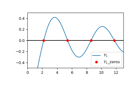

通过设置 complex=True 计算 \(Y_1\) 的前 4 个复数根和根处的导数：

>>> y1_zeros(4, True)
(array([ -0.50274327+0.78624371j,  -3.83353519+0.56235654j,
         -7.01590368+0.55339305j, -10.17357383+0.55127339j]),
 array([-0.45952768+1.31710194j,  0.04830191-0.69251288j,
        -0.02012695+0.51864253j,  0.011614  -0.43203296j]))