本文简要介绍 python 语言中 scipy.special.voigt_profile 的用法。
用法:
scipy.special.voigt_profile(x, sigma, gamma, out=None) = <ufunc 'voigt_profile'>#沃伊特简介。
Voigt 分布是具有标准差
sigma的一维正态分布和 half-width 处的一维柯西分布 (half-maximumgamma) 的卷积。如果
sigma = 0,则返回柯西分布的 PDF。相反,如果gamma = 0,则返回正态分布的 PDF。如果sigma = gamma = 0,则x = 0的返回值为Inf,所有其他x的返回值为0。- x: array_like
真正的参数
- sigma: array_like
正态分布部分的标准差
- gamma: array_like
柯西分布部分的half-maximum处的half-width
- out: ndarray,可选
函数值的可选输出数组
- 标量或 ndarray
给定参数处的 Voigt 剖面
参数 ::
返回 ::
注意:
可以用 Faddeeva 函数来表示
其中 是 Faddeeva 函数。
参考:
例子:
计算
sigma=1和gamma=1在点 2 处的函数。>>> from scipy.special import voigt_profile >>> import numpy as np >>> import matplotlib.pyplot as plt >>> voigt_profile(2, 1., 1.) 0.09071519942627544通过为 x 提供 NumPy 数组来计算多个点的函数。
>>> values = np.array([-2., 0., 5])
>>> voigt_profile(values, 1., 1.)
array([0.0907152 , 0.20870928, 0.01388492])
绘制不同参数集的函数。
>>> fig, ax = plt.subplots(figsize=(8, 8))
>>> x = np.linspace(-10, 10, 500)
>>> parameters_list = [(1.5, 0., "solid"), (1.3, 0.5, "dashed"),
...                    (0., 1.8, "dotted"), (1., 1., "dashdot")]
>>> for params in parameters_list:
...     sigma, gamma, linestyle = params
...     voigt = voigt_profile(x, sigma, gamma)
...     ax.plot(x, voigt, label=rf"$\sigma={sigma},\, \gamma={gamma}$",
...             ls=linestyle)
>>> ax.legend()
>>> plt.show()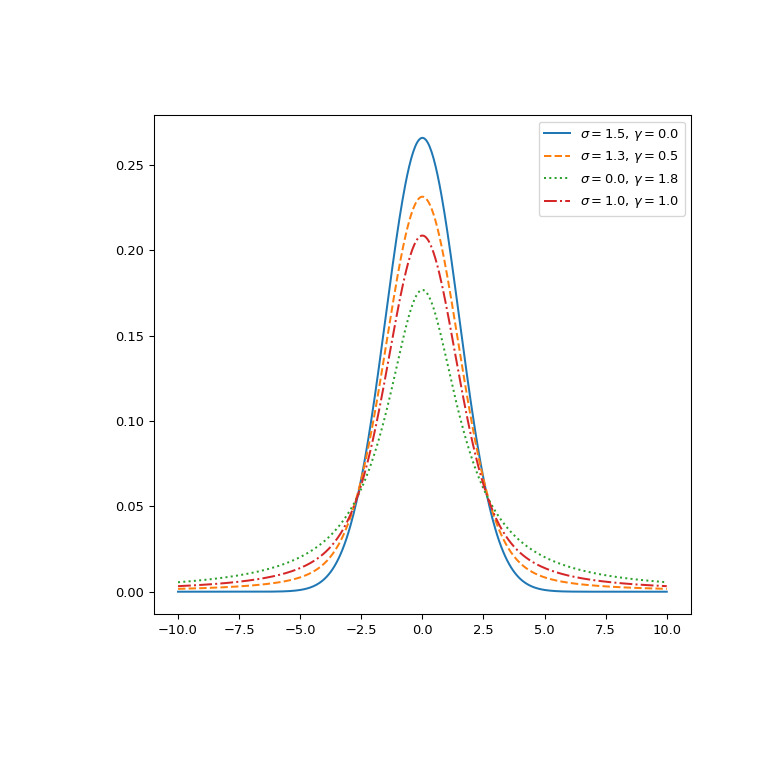
目视验证 Voigt 分布确实是作为正态分布和柯西分布的卷积而出现的。
>>> from scipy.signal import convolve
>>> x, dx = np.linspace(-10, 10, 500, retstep=True)
>>> def gaussian(x, sigma):
...     return np.exp(-0.5 * x**2/sigma**2)/(sigma * np.sqrt(2*np.pi))
>>> def cauchy(x, gamma):
...     return gamma/(np.pi * (np.square(x)+gamma**2))
>>> sigma = 2
>>> gamma = 1
>>> gauss_profile = gaussian(x, sigma)
>>> cauchy_profile = cauchy(x, gamma)
>>> convolved = dx * convolve(cauchy_profile, gauss_profile, mode="same")
>>> voigt = voigt_profile(x, sigma, gamma)
>>> fig, ax = plt.subplots(figsize=(8, 8))
>>> ax.plot(x, gauss_profile, label="Gauss: $G$", c='b')
>>> ax.plot(x, cauchy_profile, label="Cauchy: $C$", c='y', ls="dashed")
>>> xx = 0.5*(x[1:] + x[:-1])  # midpoints
>>> ax.plot(xx, convolved[1:], label="Convolution: $G * C$", ls='dashdot',
...         c='k')
>>> ax.plot(x, voigt, label="Voigt", ls='dotted', c='r')
>>> ax.legend()
>>> plt.show()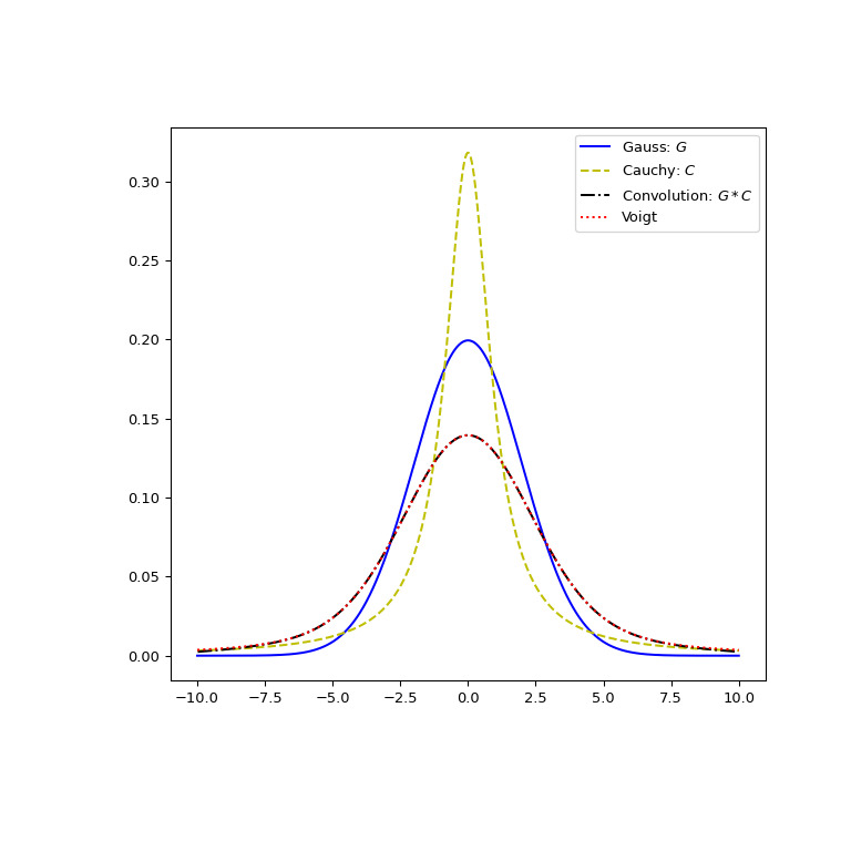
相关用法
- Python SciPy special.exp1用法及代码示例
- Python SciPy special.expn用法及代码示例
- Python SciPy special.ncfdtri用法及代码示例
- Python SciPy special.gamma用法及代码示例
- Python SciPy special.y1用法及代码示例
- Python SciPy special.y0用法及代码示例
- Python SciPy special.ellip_harm_2用法及代码示例
- Python SciPy special.i1e用法及代码示例
- Python SciPy special.smirnovi用法及代码示例
- Python SciPy special.ker用法及代码示例
- Python SciPy special.ynp_zeros用法及代码示例
- Python SciPy special.k0e用法及代码示例
- Python SciPy special.j1用法及代码示例
- Python SciPy special.logsumexp用法及代码示例
- Python SciPy special.expit用法及代码示例
- Python SciPy special.polygamma用法及代码示例
- Python SciPy special.nbdtrik用法及代码示例
- Python SciPy special.nbdtrin用法及代码示例
- Python SciPy special.seterr用法及代码示例
- Python SciPy special.ncfdtr用法及代码示例
- Python SciPy special.pdtr用法及代码示例
- Python SciPy special.expm1用法及代码示例
- Python SciPy special.shichi用法及代码示例
- Python SciPy special.smirnov用法及代码示例
- Python SciPy special.stdtr用法及代码示例
注:本文由纯净天空筛选整理自scipy.org大神的英文原创作品 scipy.special.voigt_profile。非经特殊声明,原始代码版权归原作者所有,本译文未经允许或授权,请勿转载或复制。