本文简要介绍 python 语言中 scipy.special.smirnov 的用法。
用法:
scipy.special.smirnov(n, d, out=None) = <ufunc 'smirnov'>#Kolmogorov-Smirnov互补累积分布函数
返回 Dn+(或 Dn-)的精确 Kolmogorov-Smirnov 互补累积分布函数(也称为生存函数),用于对经验分布和理论分布之间的相等性进行单方面检验。它等于理论分布与基于经验的分布之间的最大差异的概率n样本大于 d。
- n: int
样本数
- d: 浮点数 数组
经验 CDF (ECDF) 和目标 CDF 之间的偏差。
- out: ndarray,可选
函数结果的可选输出数组
- 标量或 ndarray
smirnov(n, d) 的值,Prob(Dn+ >= d) (Also Prob(Dn- >= d))
参数 ::
返回 ::
注意:
smirnov被使用stats.kstest在Kolmogorov-Smirnov 拟合优度检验的应用中。由于历史原因,此函数在scpy.special,但实现最准确的 CDF/SF/PDF/PPF/ISF 计算的推荐方法是使用stats.ksone分配。例子:
>>> import numpy as np
>>> from scipy.special import smirnov
>>> from scipy.stats import norm
显示大小为 5 的样本中差距至少为 0、0.5 和 1.0 的概率。
>>> smirnov(5, [0, 0.5, 1.0])
array([ 1.   ,  0.056,  0.   ])
将大小为 5 的样本与平均值 0、标准差 1 的标准正态分布 N(0, 1) 进行比较。
x 是样本。
>>> x = np.array([-1.392, -0.135, 0.114, 0.190, 1.82])>>> target = norm(0, 1) >>> cdfs = target.cdf(x) >>> cdfs array([0.0819612 , 0.44630594, 0.5453811 , 0.57534543, 0.9656205 ])构建经验 CDF 和 K-S 统计数据(Dn+、Dn-、Dn)。
>>> n = len(x)
>>> ecdfs = np.arange(n+1, dtype=float)/n
>>> cols = np.column_stack([x, ecdfs[1:], cdfs, cdfs - ecdfs[:n],
...                        ecdfs[1:] - cdfs])
>>> with np.printoptions(precision=3):
...    print(cols)
[[-1.392  0.2    0.082  0.082  0.118]
 [-0.135  0.4    0.446  0.246 -0.046]
 [ 0.114  0.6    0.545  0.145  0.055]
 [ 0.19   0.8    0.575 -0.025  0.225]
 [ 1.82   1.     0.966  0.166  0.034]]
>>> gaps = cols[:, -2:]
>>> Dnpm = np.max(gaps, axis=0)
>>> print(f'Dn-={Dnpm[0]:f}, Dn+={Dnpm[1]:f}')
Dn-=0.246306, Dn+=0.224655
>>> probs = smirnov(n, Dnpm)
>>> print(f'For a sample of size {n} drawn from N(0, 1):',
...       f' Smirnov n={n}: Prob(Dn- >= {Dnpm[0]:f}) = {probs[0]:.4f}',
...       f' Smirnov n={n}: Prob(Dn+ >= {Dnpm[1]:f}) = {probs[1]:.4f}',
...       sep='\n')
For a sample of size 5 drawn from N(0, 1):
 Smirnov n=5: Prob(Dn- >= 0.246306) = 0.4711
 Smirnov n=5: Prob(Dn+ >= 0.224655) = 0.5245
绘制经验 CDF 和标准正态 CDF。
>>> import matplotlib.pyplot as plt
>>> plt.step(np.concatenate(([-2.5], x, [2.5])),
...          np.concatenate((ecdfs, [1])),
...          where='post', label='Empirical CDF')
>>> xx = np.linspace(-2.5, 2.5, 100)
>>> plt.plot(xx, target.cdf(xx), '--', label='CDF for N(0, 1)')
添加标记 Dn+ 和 Dn- 的垂直线。
>>> iminus, iplus = np.argmax(gaps, axis=0)
>>> plt.vlines([x[iminus]], ecdfs[iminus], cdfs[iminus], color='r',
...            alpha=0.5, lw=4)
>>> plt.vlines([x[iplus]], cdfs[iplus], ecdfs[iplus+1], color='m',
...            alpha=0.5, lw=4)
>>> plt.grid(True) >>> plt.legend(framealpha=1, shadow=True) >>> plt.show()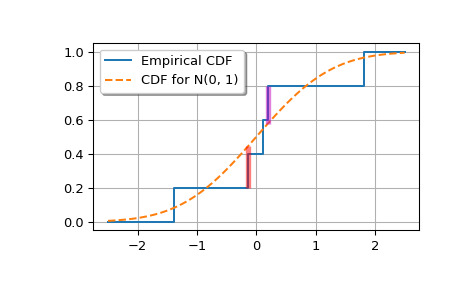
相关用法
- Python SciPy special.smirnovi用法及代码示例
- Python SciPy special.seterr用法及代码示例
- Python SciPy special.shichi用法及代码示例
- Python SciPy special.stdtr用法及代码示例
- Python SciPy special.softmax用法及代码示例
- Python SciPy special.sinc用法及代码示例
- Python SciPy special.stdtridf用法及代码示例
- Python SciPy special.sindg用法及代码示例
- Python SciPy special.spherical_kn用法及代码示例
- Python SciPy special.spherical_yn用法及代码示例
- Python SciPy special.struve用法及代码示例
- Python SciPy special.sici用法及代码示例
- Python SciPy special.spherical_in用法及代码示例
- Python SciPy special.spherical_jn用法及代码示例
- Python SciPy special.stirling2用法及代码示例
- Python SciPy special.spence用法及代码示例
- Python SciPy special.stdtrit用法及代码示例
- Python SciPy special.exp1用法及代码示例
- Python SciPy special.expn用法及代码示例
- Python SciPy special.ncfdtri用法及代码示例
- Python SciPy special.gamma用法及代码示例
- Python SciPy special.y1用法及代码示例
- Python SciPy special.y0用法及代码示例
- Python SciPy special.ellip_harm_2用法及代码示例
- Python SciPy special.i1e用法及代码示例
注:本文由纯净天空筛选整理自scipy.org大神的英文原创作品 scipy.special.smirnov。非经特殊声明,原始代码版权归原作者所有,本译文未经允许或授权,请勿转载或复制。