Python SciPy special.stdtr用法及代码示例

本文简要介绍 python 语言中 scipy.special.stdtr 的用法。

用法:

scipy.special.stdtr(df, t, out=None) = <ufunc 'stdtr'>#

学生 t 分布 累积分布函数

返回积分：

\[\frac{\Gamma((df+1)/2)}{\sqrt{\pi df} \Gamma(df/2)} \int_{-\infty}^t (1+x^2/df)^{-(df+1)/2}\, dx\]

参数 ：：

df： array_like

自由度

t： array_like

积分的上限

out： ndarray，可选

函数结果的可选输出数组

返回 ：：

标量或 ndarray

学生 t CDF 在 t 时的值

注意：

学生 t 分布也可作为 scipy.stats.t 获得。与 scipy.stats.t 的 cdf 方法相比，直接调用 stdtr 可以提高性能(请参见下面的最后一个示例)。

例子：

计算 t=1 处 df=3 的函数。

>>> import numpy as np
>>> from scipy.special import stdtr
>>> import matplotlib.pyplot as plt
>>> stdtr(3, 1)
0.8044988905221148

绘制三个不同自由度的函数。

>>> x = np.linspace(-10, 10, 1000)
>>> fig, ax = plt.subplots()
>>> parameters = [(1, "solid"), (3, "dashed"), (10, "dotted")]
>>> for (df, linestyle) in parameters:
...     ax.plot(x, stdtr(df, x), ls=linestyle, label=f"$df={df}$")
>>> ax.legend()
>>> ax.set_title("Student t distribution cumulative distribution function")
>>> plt.show()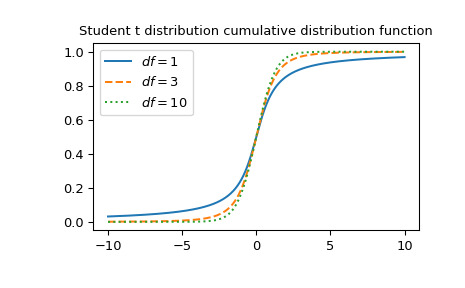

通过为 df 提供 NumPy 数组或列表，可以同时计算多个自由度的函数：

>>> stdtr([1, 2, 3], 1)
array([0.75      , 0.78867513, 0.80449889])

通过提供数组，可以同时计算多个不同自由度的多个点的函数df和t具有与广播兼容的形状。计算stdtr3 个自由度的 4 个点，形成 3x4 形状的数组。

>>> dfs = np.array([[1], [2], [3]])
>>> t = np.array([2, 4, 6, 8])
>>> dfs.shape, t.shape
((3, 1), (4,))

>>> stdtr(dfs, t)
array([[0.85241638, 0.92202087, 0.94743154, 0.96041658],
       [0.90824829, 0.97140452, 0.98666426, 0.99236596],
       [0.93033702, 0.98599577, 0.99536364, 0.99796171]])

t 分布也可用作 scipy.stats.t 。直接调用 stdtr 比调用 scipy.stats.t 的 cdf 方法要快得多。为了获得相同的结果，必须使用以下参数化：scipy.stats.t(df).cdf(x) = stdtr(df, x)。

>>> from scipy.stats import t
>>> df, x = 3, 1
>>> stdtr_result = stdtr(df, x)  # this can be faster than below
>>> stats_result = t(df).cdf(x)
>>> stats_result == stdtr_result  # test that results are equal
True