本文简要介绍 python 语言中 scipy.special.pseudo_huber 的用法。
用法:
scipy.special.pseudo_huber(delta, r, out=None) = <ufunc 'pseudo_huber'>#Pseudo-Huber损失函数。
- delta: array_like
输入数组,指示软二次与线性损耗变化点。
- r: array_like
输入数组,可能表示残差。
- out: ndarray,可选
函数结果的可选输出数组
- res: 标量或 ndarray
计算出的Pseudo-Huber损失函数值。
参数 ::
返回 ::
注意:
与
huber一样,pseudo_huber通常用作统计或机器学习中的稳健损失函数,以减少异常值的影响。与huber不同,pseudo_huber很平滑。通常,r表示残差,即模型预测与数据之间的差异。那么,对于,
pseudo_huber类似于平方误差并且对于绝对误差。这样,Pseudo-Huber 损失通常可以在像平方误差损失函数这样的小残差模型拟合中实现快速收敛,并且仍然减少异常值的影响()就像绝对误差损失一样。作为是平方误差范围和绝对误差范围之间的分界线,必须针对每个问题仔细调整。pseudo_huber也是凸的,使其适合基于梯度的优化。[1] [2]参考:
[1]Hartley、Zisserman,“计算机视觉中的多视图几何”。 2003。剑桥大学出版社。 p。 619
[2]沙博尼耶等人。 “计算成像中的确定性edge-preserving正则化”。 1997. IEEE 传输。图像处理。 6(2):298-311。
例子:
导入所有必需的模块。
>>> import numpy as np
>>> from scipy.special import pseudo_huber, huber
>>> import matplotlib.pyplot as plt
计算
r=2处delta=1的函数。>>> pseudo_huber(1., 2.) 1.2360679774997898计算函数在
r=2对于不同的三角洲通过提供列表或NumPy数组三角洲.>>> pseudo_huber([1., 2., 4.], 3.) array([2.16227766, 3.21110255, 4. ])计算函数为
delta=1通过提供列表或 NumPy 数组来在多个点上r.>>> pseudo_huber(2., np.array([1., 1.5, 3., 4.])) array([0.47213595, 1. , 3.21110255, 4.94427191])通过为广播提供兼容形状的数组,可以针对不同的 delta 和 r 计算该函数。
>>> r = np.array([1., 2.5, 8., 10.])
>>> deltas = np.array([[1.], [5.], [9.]])
>>> print(r.shape, deltas.shape)
(4,) (3, 1)
>>> pseudo_huber(deltas, r) array([[ 0.41421356, 1.6925824 , 7.06225775, 9.04987562], [ 0.49509757, 2.95084972, 22.16990566, 30.90169944], [ 0.49846624, 3.06693762, 27.37435121, 40.08261642]])绘制不同 delta 的函数。
>>> x = np.linspace(-4, 4, 500)
>>> deltas = [1, 2, 3]
>>> linestyles = ["dashed", "dotted", "dashdot"]
>>> fig, ax = plt.subplots()
>>> combined_plot_parameters = list(zip(deltas, linestyles))
>>> for delta, style in combined_plot_parameters:
...     ax.plot(x, pseudo_huber(delta, x), label=f"$\delta={delta}$",
...             ls=style)
>>> ax.legend(loc="upper center")
>>> ax.set_xlabel("$x$")
>>> ax.set_title("Pseudo-Huber loss function $h_{\delta}(x)$")
>>> ax.set_xlim(-4, 4)
>>> ax.set_ylim(0, 8)
>>> plt.show()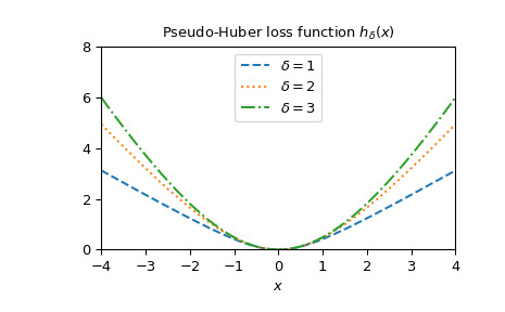
最后说明一下两者的区别
huber和pseudo_huber通过绘制它们及其相对于的梯度r。该图表明pseudo_huber是连续可微的,同时huber不在点上.>>> def huber_grad(delta, x): ... grad = np.copy(x) ... linear_area = np.argwhere(np.abs(x) > delta) ... grad[linear_area]=delta*np.sign(x[linear_area]) ... return grad >>> def pseudo_huber_grad(delta, x): ... return x* (1+(x/delta)**2)**(-0.5) >>> x=np.linspace(-3, 3, 500) >>> delta = 1. >>> fig, ax = plt.subplots(figsize=(7, 7)) >>> ax.plot(x, huber(delta, x), label="Huber", ls="dashed") >>> ax.plot(x, huber_grad(delta, x), label="Huber Gradient", ls="dashdot") >>> ax.plot(x, pseudo_huber(delta, x), label="Pseudo-Huber", ls="dotted") >>> ax.plot(x, pseudo_huber_grad(delta, x), label="Pseudo-Huber Gradient", ... ls="solid") >>> ax.legend(loc="upper center") >>> plt.show()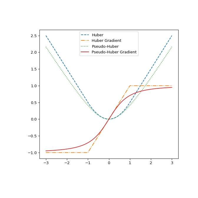
相关用法
- Python SciPy special.psi用法及代码示例
- Python SciPy special.polygamma用法及代码示例
- Python SciPy special.pdtr用法及代码示例
- Python SciPy special.powm1用法及代码示例
- Python SciPy special.poch用法及代码示例
- Python SciPy special.perm用法及代码示例
- Python SciPy special.exp1用法及代码示例
- Python SciPy special.expn用法及代码示例
- Python SciPy special.ncfdtri用法及代码示例
- Python SciPy special.gamma用法及代码示例
- Python SciPy special.y1用法及代码示例
- Python SciPy special.y0用法及代码示例
- Python SciPy special.ellip_harm_2用法及代码示例
- Python SciPy special.i1e用法及代码示例
- Python SciPy special.smirnovi用法及代码示例
- Python SciPy special.ker用法及代码示例
- Python SciPy special.ynp_zeros用法及代码示例
- Python SciPy special.k0e用法及代码示例
- Python SciPy special.j1用法及代码示例
- Python SciPy special.logsumexp用法及代码示例
- Python SciPy special.expit用法及代码示例
- Python SciPy special.nbdtrik用法及代码示例
- Python SciPy special.nbdtrin用法及代码示例
- Python SciPy special.seterr用法及代码示例
- Python SciPy special.ncfdtr用法及代码示例
注:本文由纯净天空筛选整理自scipy.org大神的英文原创作品 scipy.special.pseudo_huber。非经特殊声明,原始代码版权归原作者所有,本译文未经允许或授权,请勿转载或复制。