本文简要介绍 python 语言中 scipy.special.kolmogorov 的用法。
用法:
scipy.special.kolmogorov(y, out=None) = <ufunc 'kolmogorov'>#Kolmogorov 分布的互补累积分布(生存函数)函数。
返回经验分布和理论分布之间相等性的双边检验的柯尔莫哥洛夫极限分布(
D_n*\sqrt(n),当 n 趋于无穷大)的互补累积分布函数。它等于sqrt(n) * max absolute deviation > y的概率(限制为 n->无穷大)。- y: 浮点数 数组
经验 CDF (ECDF) 和目标 CDF 之间的绝对偏差,乘以 sqrt(n)。
- out: ndarray,可选
函数结果的可选输出数组
- 标量或 ndarray
kolmogorov(y) 的值
参数 ::
返回 ::
注意:
kolmogorov被使用stats.kstest在Kolmogorov-Smirnov 拟合优度检验的应用中。由于历史原因,此函数在scpy.special,但实现最准确的 CDF/SF/PDF/PPF/ISF 计算的推荐方法是使用stats.kstwobign分配。例子:
显示至少与 0、0.5 和 1.0 一样大的差距的概率。
>>> import numpy as np
>>> from scipy.special import kolmogorov
>>> from scipy.stats import kstwobign
>>> kolmogorov([0, 0.5, 1.0])
array([ 1.        ,  0.96394524,  0.26999967])
比较从 Laplace(0, 1) 分布中抽取的大小为 1000 的样本与目标分布,即 Normal(0, 1) 分布。
>>> from scipy.stats import norm, laplace
>>> rng = np.random.default_rng()
>>> n = 1000
>>> lap01 = laplace(0, 1)
>>> x = np.sort(lap01.rvs(n, random_state=rng))
>>> np.mean(x), np.std(x)
(-0.05841730131499543, 1.3968109101997568)
构造经验 CDF 和 K-S 统计量 Dn。
>>> target = norm(0,1)  # Normal mean 0, stddev 1
>>> cdfs = target.cdf(x)
>>> ecdfs = np.arange(n+1, dtype=float)/n
>>> gaps = np.column_stack([cdfs - ecdfs[:n], ecdfs[1:] - cdfs])
>>> Dn = np.max(gaps)
>>> Kn = np.sqrt(n) * Dn
>>> print('Dn=%f, sqrt(n)*Dn=%f' % (Dn, Kn))
Dn=0.043363, sqrt(n)*Dn=1.371265
>>> print(chr(10).join(['For a sample of size n drawn from a N(0, 1) distribution:',
...   ' the approximate Kolmogorov probability that sqrt(n)*Dn>=%f is %f' %  (Kn, kolmogorov(Kn)),
...   ' the approximate Kolmogorov probability that sqrt(n)*Dn<=%f is %f' %  (Kn, kstwobign.cdf(Kn))]))
For a sample of size n drawn from a N(0, 1) distribution:
 the approximate Kolmogorov probability that sqrt(n)*Dn>=1.371265 is 0.046533
 the approximate Kolmogorov probability that sqrt(n)*Dn<=1.371265 is 0.953467
针对目标 N(0, 1) CDF 绘制经验 CDF。
>>> import matplotlib.pyplot as plt
>>> plt.step(np.concatenate([[-3], x]), ecdfs, where='post', label='Empirical CDF')
>>> x3 = np.linspace(-3, 3, 100)
>>> plt.plot(x3, target.cdf(x3), label='CDF for N(0, 1)')
>>> plt.ylim([0, 1]); plt.grid(True); plt.legend();
>>> # Add vertical lines marking Dn+ and Dn-
>>> iminus, iplus = np.argmax(gaps, axis=0)
>>> plt.vlines([x[iminus]], ecdfs[iminus], cdfs[iminus], color='r', linestyle='dashed', lw=4)
>>> plt.vlines([x[iplus]], cdfs[iplus], ecdfs[iplus+1], color='r', linestyle='dashed', lw=4)
>>> plt.show()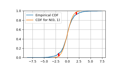
相关用法
- Python SciPy special.kolmogi用法及代码示例
- Python SciPy special.ker用法及代码示例
- Python SciPy special.k0e用法及代码示例
- Python SciPy special.kvp用法及代码示例
- Python SciPy special.kve用法及代码示例
- Python SciPy special.k1e用法及代码示例
- Python SciPy special.kv用法及代码示例
- Python SciPy special.kn用法及代码示例
- Python SciPy special.k1用法及代码示例
- Python SciPy special.k0用法及代码示例
- Python SciPy special.kei用法及代码示例
- Python SciPy special.exp1用法及代码示例
- Python SciPy special.expn用法及代码示例
- Python SciPy special.ncfdtri用法及代码示例
- Python SciPy special.gamma用法及代码示例
- Python SciPy special.y1用法及代码示例
- Python SciPy special.y0用法及代码示例
- Python SciPy special.ellip_harm_2用法及代码示例
- Python SciPy special.i1e用法及代码示例
- Python SciPy special.smirnovi用法及代码示例
- Python SciPy special.ynp_zeros用法及代码示例
- Python SciPy special.j1用法及代码示例
- Python SciPy special.logsumexp用法及代码示例
- Python SciPy special.expit用法及代码示例
- Python SciPy special.polygamma用法及代码示例
注:本文由纯净天空筛选整理自scipy.org大神的英文原创作品 scipy.special.kolmogorov。非经特殊声明,原始代码版权归原作者所有,本译文未经允许或授权,请勿转载或复制。