Python SciPy interpolate.CubicSpline用法及代碼示例

本文簡要介紹 python 語言中 scipy.interpolate.CubicSpline 的用法。

用法:

class  scipy.interpolate.CubicSpline(x, y, axis=0, bc_type='not-a-knot', extrapolate=None)#

三次樣條數據插值器。

使用兩次連續可導的分段三次多項式對數據進行插值 [1]。結果表示為 PPoly 實例，其中斷點與給定數據匹配。

參數 ：：

x： 數組, 形狀 (n,)

包含自變量值的一維數組。值必須是實數、有限且嚴格遞增的。

y： array_like

包含因變量值的數組。它可以有任意數量的維度，但沿 axis 的長度(見下文)必須與 x 的長度匹配。值必須是有限的。

axis： 整數，可選

沿哪個軸y假設是變化的。這意味著對於x[i]對應的值為np.take(y, i, axis=axis).默認值為 0。

bc_type： 字符串或 2 元組，可選

邊界條件類型。需要由邊界條件給出的兩個附加方程來確定每個段 [2] 上多項式的所有係數。

如果bc_type 是字符串，則指定的條件將應用於樣條曲線的兩端。可用條件為：

• ‘not-a-knot’(默認)：曲線末端的第一段和第二段是相同的多項式。當沒有關於邊界條件的信息時，這是一個很好的默認值。

• ‘periodic’：假設插值函數是周期性的x[-1] - x[0].的第一個和最後一個值y必須相同：y[0] == y[-1].這個邊界條件將導致y'[0] == y'[-1]和y''[0] == y''[-1].

• ‘clamped’：曲線末端的一階導數為零。假設一維y,bc_type=((1, 0.0), (1, 0.0))是相同的條件。

• ‘natural’：曲線末端的二階導數為零。假設一維y,bc_type=((2, 0.0), (2, 0.0))是相同的條件。

如果bc_type 是一個二元組，則第一個和第二個值將分別應用於曲線的起點和終點。元組值可以是前麵提到的字符串之一(‘periodic’ 除外)或允許在曲線末端指定任意導數的元組(順序，deriv_values)：

• order：導數順序，1 或 2。

• deriv_value: 數組 包含導數值，形狀必須相同y, 不包括axis方麵。例如，如果y是一維的，那麽deriv_value必須是標量。如果y是 3-D，形狀為 (n0, n1, n2) 且軸 = 2，則deriv_value必須是二維的並且具有 (n0, n1) 的形狀。

extrapolate： {bool，‘periodic’，無}，可選

如果是布爾值，則確定是根據第一個和最後一個間隔外推到越界點，還是返回 NaN。如果‘periodic’，使用周期性外推。如果 None (默認)，extrapolate 設置為 ‘periodic’ 用於 bc_type='periodic'，否則設置為 True。

注意：

參數bc_type和extrapolate獨立工作，即前者僅控製樣條的構造，而後者僅控製評估。

當邊界條件為“not-a-knot”且 n = 2 時，將其替換為一階導數等於線性插值斜率的條件。當兩個邊界條件均為“not-a-knot”且 n = 3 時，求解作為通過給定點的拋物線尋求。

當 'not-a-knot' 邊界條件應用於兩端時，生成的樣條曲線將與 splrep (使用 s=0 )和 InterpolatedUnivariateSpline 返回的樣條曲線相同，但這兩種方法使用 B-spline 基礎中的表示.

參考：

[1]

Cubic Spline Interpolation 在維基學院。

[2]

Carl de Boor，“樣條曲線實用指南”，Springer-Verlag，1978 年。

例子：

在此示例中，三次樣條用於內插采樣的正弦曲線。您可以看到樣條連續性屬性適用於一階和二階導數，僅違反三階導數。

>>> import numpy as np
>>> from scipy.interpolate import CubicSpline
>>> import matplotlib.pyplot as plt
>>> x = np.arange(10)
>>> y = np.sin(x)
>>> cs = CubicSpline(x, y)
>>> xs = np.arange(-0.5, 9.6, 0.1)
>>> fig, ax = plt.subplots(figsize=(6.5, 4))
>>> ax.plot(x, y, 'o', label='data')
>>> ax.plot(xs, np.sin(xs), label='true')
>>> ax.plot(xs, cs(xs), label="S")
>>> ax.plot(xs, cs(xs, 1), label="S'")
>>> ax.plot(xs, cs(xs, 2), label="S''")
>>> ax.plot(xs, cs(xs, 3), label="S'''")
>>> ax.set_xlim(-0.5, 9.5)
>>> ax.legend(loc='lower left', ncol=2)
>>> plt.show()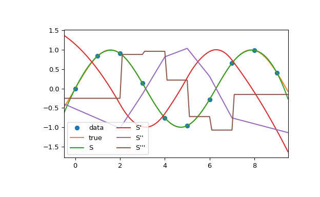

在第二個例子中，單位圓是用樣條插值的。使用周期性邊界條件。您可以看到周期點 (1, 0) 處的一階導數值 ds/dx=0, ds/dy=1 被正確計算。請注意，圓不能用三次樣條精確表示。為了提高精度，需要更多的斷點。

>>> theta = 2 * np.pi * np.linspace(0, 1, 5)
>>> y = np.c_[np.cos(theta), np.sin(theta)]
>>> cs = CubicSpline(theta, y, bc_type='periodic')
>>> print("ds/dx={:.1f} ds/dy={:.1f}".format(cs(0, 1)[0], cs(0, 1)[1]))
ds/dx=0.0 ds/dy=1.0
>>> xs = 2 * np.pi * np.linspace(0, 1, 100)
>>> fig, ax = plt.subplots(figsize=(6.5, 4))
>>> ax.plot(y[:, 0], y[:, 1], 'o', label='data')
>>> ax.plot(np.cos(xs), np.sin(xs), label='true')
>>> ax.plot(cs(xs)[:, 0], cs(xs)[:, 1], label='spline')
>>> ax.axes.set_aspect('equal')
>>> ax.legend(loc='center')
>>> plt.show()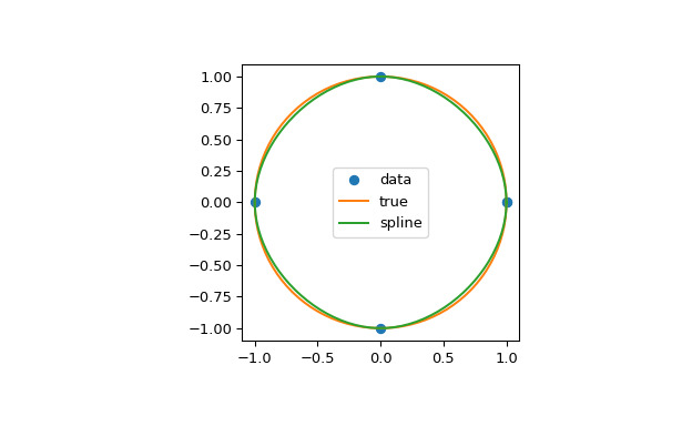

第三個例子是多項式 y = x**3 在區間 0 <= x<= 1 上的插值。三次樣條可以精確地表示這個函數。為了實現這一點，我們需要在區間的端點處指定值和一階導數。請注意，y' = 3 * x**2，因此 y'(0) = 0 和 y'(1) = 3。

>>> cs = CubicSpline([0, 1], [0, 1], bc_type=((1, 0), (1, 3)))
>>> x = np.linspace(0, 1)
>>> np.allclose(x**3, cs(x))
True

屬性 ：：

x： ndarray，形狀(n，)

斷點。傳遞給構造函數的相同x。

c： ndarray，形狀(4，n-1，...)

每個段上多項式的係數。尾隨尺寸與y, 不包括axis.例如，如果y是一維，那麽c[k, i]是一個係數(x-x[i])**(3-k)在之間的段x[i]和x[i+1].

axis： int

插值軸。傳遞給構造函數的同一軸。