Tidy 总结了有关模型组件的信息。模型组件可能是回归中的单个项、单个假设、聚类或类。 tidy 所认为的模型组件的确切含义因模型而异,但通常是不言而喻的。如果模型具有多种不同类型的组件,您将需要指定要返回哪些组件。
参数
- x
-
从
survival::survreg()返回的survreg对象。 - conf.level
-
用于置信区间的置信水平(如果
conf.int = TRUE)。必须严格大于 0 且小于 1。默认为 0.95,对应于 95% 的置信区间。 - conf.int
-
逻辑指示是否在整理的输出中包含置信区间。默认为
FALSE。 - ...
-
附加参数。不曾用过。仅需要匹配通用签名。注意:拼写错误的参数将被吸收到
...中,并被忽略。如果拼写错误的参数有默认值,则将使用默认值。例如,如果您传递conf.lvel = 0.9,所有计算将使用conf.level = 0.95进行。这里有两个异常:
也可以看看
其他 survreg 整理器:augment.survreg() 、glance.survreg()
其他生存整理器:augment.coxph() , augment.survreg() , glance.aareg() , glance.cch() , glance.coxph() , glance.pyears() , glance.survdiff() , glance.survexp() , glance.survfit() , glance.survreg() , tidy.aareg() , tidy.cch() , tidy.coxph() , tidy.pyears() , tidy.survdiff() , tidy.survexp() , tidy.survfit()
值
带有列的 tibble::tibble():
- conf.high
-
估计置信区间的上限。
- conf.low
-
估计置信区间的下限。
- estimate
-
回归项的估计值。
- p.value
-
与观察到的统计量相关的两侧 p 值。
- statistic
-
在回归项非零的假设中使用的 T-statistic 的值。
- std.error
-
回归项的标准误差。
- term
-
回归项的名称。
例子
# load libraries for models and data
library(survival)
# fit model
sr <- survreg(
Surv(futime, fustat) ~ ecog.ps + rx,
ovarian,
dist = "exponential"
)
# summarize model fit with tidiers + visualization
tidy(sr)
#> # A tibble: 3 × 5
#> term estimate std.error statistic p.value
#> <chr> <dbl> <dbl> <dbl> <dbl>
#> 1 (Intercept) 6.96 1.32 5.27 0.000000139
#> 2 ecog.ps -0.433 0.587 -0.738 0.461
#> 3 rx 0.582 0.587 0.991 0.322
augment(sr, ovarian)
#> # A tibble: 26 × 9
#> futime fustat age resid.ds rx ecog.ps .fitted .se.fit .resid
#> <dbl> <dbl> <dbl> <dbl> <dbl> <dbl> <dbl> <dbl> <dbl>
#> 1 59 1 72.3 2 1 1 1224. 639. -1165.
#> 2 115 1 74.5 2 1 1 1224. 639. -1109.
#> 3 156 1 66.5 2 1 2 794. 350. -638.
#> 4 421 0 53.4 2 2 1 2190. 1202. -1769.
#> 5 431 1 50.3 2 1 1 1224. 639. -793.
#> 6 448 0 56.4 1 1 2 794. 350. -346.
#> 7 464 1 56.9 2 2 2 1420. 741. -956.
#> 8 475 1 59.9 2 2 2 1420. 741. -945.
#> 9 477 0 64.2 2 1 1 1224. 639. -747.
#> 10 563 1 55.2 1 2 2 1420. 741. -857.
#> # ℹ 16 more rows
glance(sr)
#> # A tibble: 1 × 9
#> iter df statistic logLik AIC BIC df.residual nobs p.value
#> <int> <int> <dbl> <dbl> <dbl> <dbl> <int> <int> <dbl>
#> 1 4 3 1.67 -97.2 200. 204. 23 26 0.434
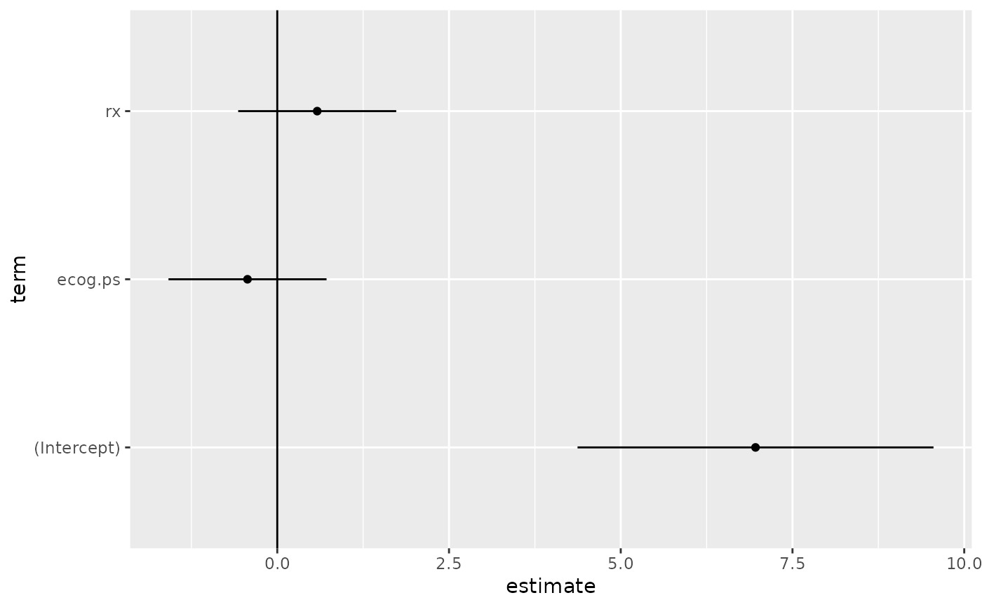
# coefficient plot
td <- tidy(sr, conf.int = TRUE)
library(ggplot2)
ggplot(td, aes(estimate, term)) +
geom_point() +
geom_errorbarh(aes(xmin = conf.low, xmax = conf.high), height = 0) +
geom_vline(xintercept = 0)
相关用法
- R broom tidy.survexp 整理 a(n) survexp 对象
- R broom tidy.survdiff 整理 a(n) survdiff 对象
- R broom tidy.survfit 整理 a(n) survfit 对象
- R broom tidy.summary_emm 整理一个(n)summary_emm对象
- R broom tidy.summary.glht 整理一个(n)summary.glht对象
- R broom tidy.summary.lm 整理 a(n)summary.lm 对象
- R broom tidy.svyolr 整理 a(n) svyolr 对象
- R broom tidy.spec 整理一个(n)规范对象
- R broom tidy.sarlm 空间自回归模型的整理方法
- R broom tidy.speedglm 整理 a(n) speedglm 对象
- R broom tidy.speedlm 整理 a(n) speedlm 对象
- R broom tidy.systemfit 整理 a(n) systemfit 对象
- R broom tidy.robustbase.glmrob 整理 a(n) glmrob 对象
- R broom tidy.acf 整理 a(n) acf 对象
- R broom tidy.robustbase.lmrob 整理 a(n) lmrob 对象
- R broom tidy.biglm 整理 a(n) biglm 对象
- R broom tidy.garch 整理 a(n) garch 对象
- R broom tidy.rq 整理 a(n) rq 对象
- R broom tidy.kmeans 整理 a(n) kmeans 对象
- R broom tidy.betamfx 整理 a(n) betamfx 对象
- R broom tidy.anova 整理 a(n) anova 对象
- R broom tidy.btergm 整理 a(n) btergm 对象
- R broom tidy.cv.glmnet 整理 a(n) cv.glmnet 对象
- R broom tidy.roc 整理 a(n) roc 对象
- R broom tidy.poLCA 整理 a(n) poLCA 对象
注:本文由纯净天空筛选整理自等大神的英文原创作品 Tidy a(n) survreg object。非经特殊声明,原始代码版权归原作者所有,本译文未经允许或授权,请勿转载或复制。