Tidy 总结了有关模型组件的信息。模型组件可能是回归中的单个项、单个假设、聚类或类。 tidy 所认为的模型组件的确切含义因模型而异,但通常是不言而喻的。如果模型具有多种不同类型的组件,您将需要指定要返回哪些组件。
参数
- x
-
从
survival::coxph()返回的coxph对象。 - exponentiate
-
逻辑指示是否对系数估计值取幂。这对于逻辑回归和多项回归来说是典型的,但如果没有 log 或 logit 链接,那么这是一个坏主意。默认为
FALSE。 - conf.int
-
逻辑指示是否在整理的输出中包含置信区间。默认为
FALSE。 - conf.level
-
用于置信区间的置信水平(如果
conf.int = TRUE)。必须严格大于 0 且小于 1。默认为 0.95,对应于 95% 的置信区间。 - ...
-
对于
tidy(),附加参数传递给summary(x, ...)。否则忽略。
也可以看看
其他 coxph 整理器:augment.coxph()、glance.coxph()
其他生存整理器:augment.coxph() , augment.survreg() , glance.aareg() , glance.cch() , glance.coxph() , glance.pyears() , glance.survdiff() , glance.survexp() , glance.survfit() , glance.survreg() , tidy.aareg() , tidy.cch() , tidy.pyears() , tidy.survdiff() , tidy.survexp() , tidy.survfit() , tidy.survreg()
值
带有列的 tibble::tibble():
- estimate
-
回归项的估计值。
- p.value
-
与观察到的统计量相关的两侧 p 值。
- statistic
-
在回归项非零的假设中使用的 T-statistic 的值。
- std.error
-
回归项的标准误差。
例子
# load libraries for models and data
library(survival)
# fit model
cfit <- coxph(Surv(time, status) ~ age + sex, lung)
# summarize model fit with tidiers
tidy(cfit)
#> # A tibble: 2 × 5
#> term estimate std.error statistic p.value
#> <chr> <dbl> <dbl> <dbl> <dbl>
#> 1 age 0.0170 0.00922 1.85 0.0646
#> 2 sex -0.513 0.167 -3.06 0.00218
tidy(cfit, exponentiate = TRUE)
#> # A tibble: 2 × 5
#> term estimate std.error statistic p.value
#> <chr> <dbl> <dbl> <dbl> <dbl>
#> 1 age 1.02 0.00922 1.85 0.0646
#> 2 sex 0.599 0.167 -3.06 0.00218
lp <- augment(cfit, lung)
risks <- augment(cfit, lung, type.predict = "risk")
expected <- augment(cfit, lung, type.predict = "expected")
glance(cfit)
#> # A tibble: 1 × 18
#> n nevent statistic.log p.value.log statistic.sc p.value.sc
#> <int> <dbl> <dbl> <dbl> <dbl> <dbl>
#> 1 228 165 14.1 0.000857 13.7 0.00105
#> # ℹ 12 more variables: statistic.wald <dbl>, p.value.wald <dbl>,
#> # statistic.robust <dbl>, p.value.robust <dbl>, r.squared <dbl>,
#> # r.squared.max <dbl>, concordance <dbl>, std.error.concordance <dbl>,
#> # logLik <dbl>, AIC <dbl>, BIC <dbl>, nobs <int>
# also works on clogit models
resp <- levels(logan$occupation)
n <- nrow(logan)
indx <- rep(1:n, length(resp))
logan2 <- data.frame(
logan[indx, ],
id = indx,
tocc = factor(rep(resp, each = n))
)
logan2$case <- (logan2$occupation == logan2$tocc)
cl <- clogit(case ~ tocc + tocc:education + strata(id), logan2)
tidy(cl)
#> # A tibble: 9 × 5
#> term estimate std.error statistic p.value
#> <chr> <dbl> <dbl> <dbl> <dbl>
#> 1 toccfarm -1.90 1.38 -1.37 1.70e- 1
#> 2 toccoperatives 1.17 0.566 2.06 3.91e- 2
#> 3 toccprofessional -8.10 0.699 -11.6 4.45e-31
#> 4 toccsales -5.03 0.770 -6.53 6.54e-11
#> 5 tocccraftsmen:education -0.332 0.0569 -5.84 5.13e- 9
#> 6 toccfarm:education -0.370 0.116 -3.18 1.47e- 3
#> 7 toccoperatives:education -0.422 0.0584 -7.23 4.98e-13
#> 8 toccprofessional:education 0.278 0.0510 5.45 4.94e- 8
#> 9 toccsales:education NA 0 NA NA
glance(cl)
#> # A tibble: 1 × 18
#> n nevent statistic.log p.value.log statistic.sc p.value.sc
#> <int> <dbl> <dbl> <dbl> <dbl> <dbl>
#> 1 4190 838 666. 1.90e-138 682. 5.01e-142
#> # ℹ 12 more variables: statistic.wald <dbl>, p.value.wald <dbl>,
#> # statistic.robust <dbl>, p.value.robust <dbl>, r.squared <dbl>,
#> # r.squared.max <dbl>, concordance <dbl>, std.error.concordance <dbl>,
#> # logLik <dbl>, AIC <dbl>, BIC <dbl>, nobs <int>
library(ggplot2)
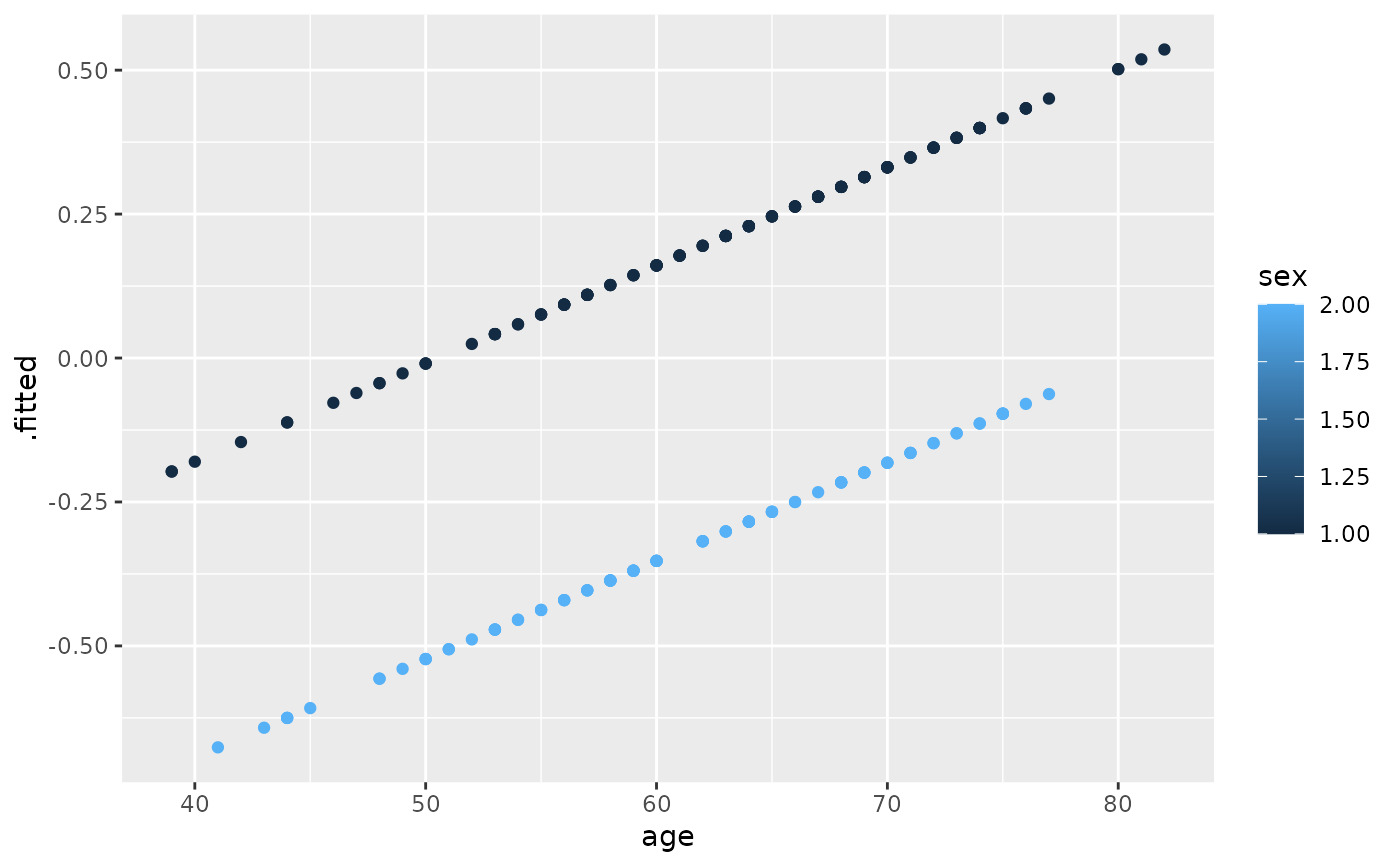
ggplot(lp, aes(age, .fitted, color = sex)) +
geom_point()
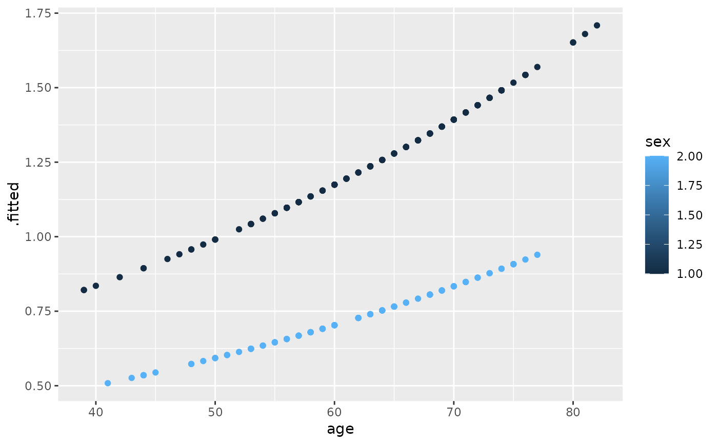
 ggplot(risks, aes(age, .fitted, color = sex)) +
geom_point()
ggplot(risks, aes(age, .fitted, color = sex)) +
geom_point()
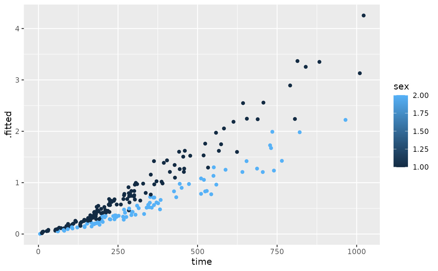
 ggplot(expected, aes(time, .fitted, color = sex)) +
geom_point()
ggplot(expected, aes(time, .fitted, color = sex)) +
geom_point()
相关用法
- R broom tidy.coeftest 整理 a(n) coeftest 对象
- R broom tidy.confint.glht 整理 a(n) confint.glht 对象
- R broom tidy.confusionMatrix 整理一个(n)confusionMatrix对象
- R broom tidy.cv.glmnet 整理 a(n) cv.glmnet 对象
- R broom tidy.cch 整理 a(n) cch 对象
- R broom tidy.cld 整理 a(n) cld 对象
- R broom tidy.clmm 整理 a(n) clmm 对象
- R broom tidy.clm 整理 a(n) clm 对象
- R broom tidy.crr 整理 a(n) cmprsk 对象
- R broom tidy.robustbase.glmrob 整理 a(n) glmrob 对象
- R broom tidy.acf 整理 a(n) acf 对象
- R broom tidy.robustbase.lmrob 整理 a(n) lmrob 对象
- R broom tidy.biglm 整理 a(n) biglm 对象
- R broom tidy.garch 整理 a(n) garch 对象
- R broom tidy.rq 整理 a(n) rq 对象
- R broom tidy.kmeans 整理 a(n) kmeans 对象
- R broom tidy.betamfx 整理 a(n) betamfx 对象
- R broom tidy.anova 整理 a(n) anova 对象
- R broom tidy.btergm 整理 a(n) btergm 对象
- R broom tidy.roc 整理 a(n) roc 对象
- R broom tidy.poLCA 整理 a(n) poLCA 对象
- R broom tidy.emmGrid 整理 a(n) emmGrid 对象
- R broom tidy.Kendall 整理 a(n) Kendall 对象
- R broom tidy.survreg 整理 a(n) survreg 对象
- R broom tidy.ergm 整理 a(n) ergm 对象
注:本文由纯净天空筛选整理自等大神的英文原创作品 Tidy a(n) coxph object。非经特殊声明,原始代码版权归原作者所有,本译文未经允许或授权,请勿转载或复制。