将每个级别映射到色轮上均匀间隔的色调。它不会生成colour-blind安全调色板。
用法
scale_colour_hue(
  ...,
  h = c(0, 360) + 15,
  c = 100,
  l = 65,
  h.start = 0,
  direction = 1,
  na.value = "grey50",
  aesthetics = "colour"
)

scale_fill_hue(
  ...,
  h = c(0, 360) + 15,
  c = 100,
  l = 65,
  h.start = 0,
  direction = 1,
  na.value = "grey50",
  aesthetics = "fill"
)
参数
- ...
-
参数传递给
discrete_scalepalette-
调色板函数,当使用单个整数参数(比例中的级别数)调用时,返回它们应采用的值(例如
scales::hue_pal())。 breaks-
之一:
limits-
之一:
-
NULL使用默认比例值 -
定义可能的比例值及其顺序的字符向量
-
接受现有(自动)值并返回新值的函数。还接受 rlang lambda 函数表示法。
-
drop-
是否应该从量表中省略未使用的因子水平?默认值
TRUE使用数据中出现的级别;FALSE使用因子中的所有级别。 na.translate-
与连续尺度不同,离散尺度可以轻松显示缺失值,并且默认情况下会这样做。如果要从离散尺度中删除缺失值,请指定
na.translate = FALSE。 scale_name-
应用于与该比例关联的错误消息的比例名称。
name-
秤的名称。用作轴或图例标题。如果
waiver()(默认值),则比例名称取自用于该美学的第一个映射。如果是NULL,则图例标题将被省略。 labels-
之一:
guide-
用于创建指南或其名称的函数。有关详细信息,请参阅
guides()。 expand-
对于位置刻度,范围扩展常量的向量,用于在数据周围添加一些填充,以确保它们放置在距轴一定距离的位置。使用便捷函数
expansion()生成expand参数的值。默认情况下,对于连续变量,每侧扩展 5%,对于离散变量,每侧扩展 0.6 个单位。 position-
对于位置刻度,轴的位置。
left或right表示 y 轴,top或bottom表示 x 轴。 super-
用于构造比例的超类
- h
-
要使用的色调范围,在 [0, 360] 中
- c
-
色度(颜色的强度),最大值根据色调和亮度的组合而变化。
- l
-
亮度(亮度),单位为 [0, 100]
- h.start
-
色调开始于
- direction
-
绕色轮移动的方向,1 = 顺时针,-1 = 逆时针
- na.value
-
用于缺失值的颜色
- aesthetics
-
字符串或字符串向量,列出了该比例所使用的美学名称。例如,这可以用于通过
aesthetics = c("colour", "fill")同时将颜色设置应用于colour和fill美学。
例子
# \donttest{
set.seed(596)
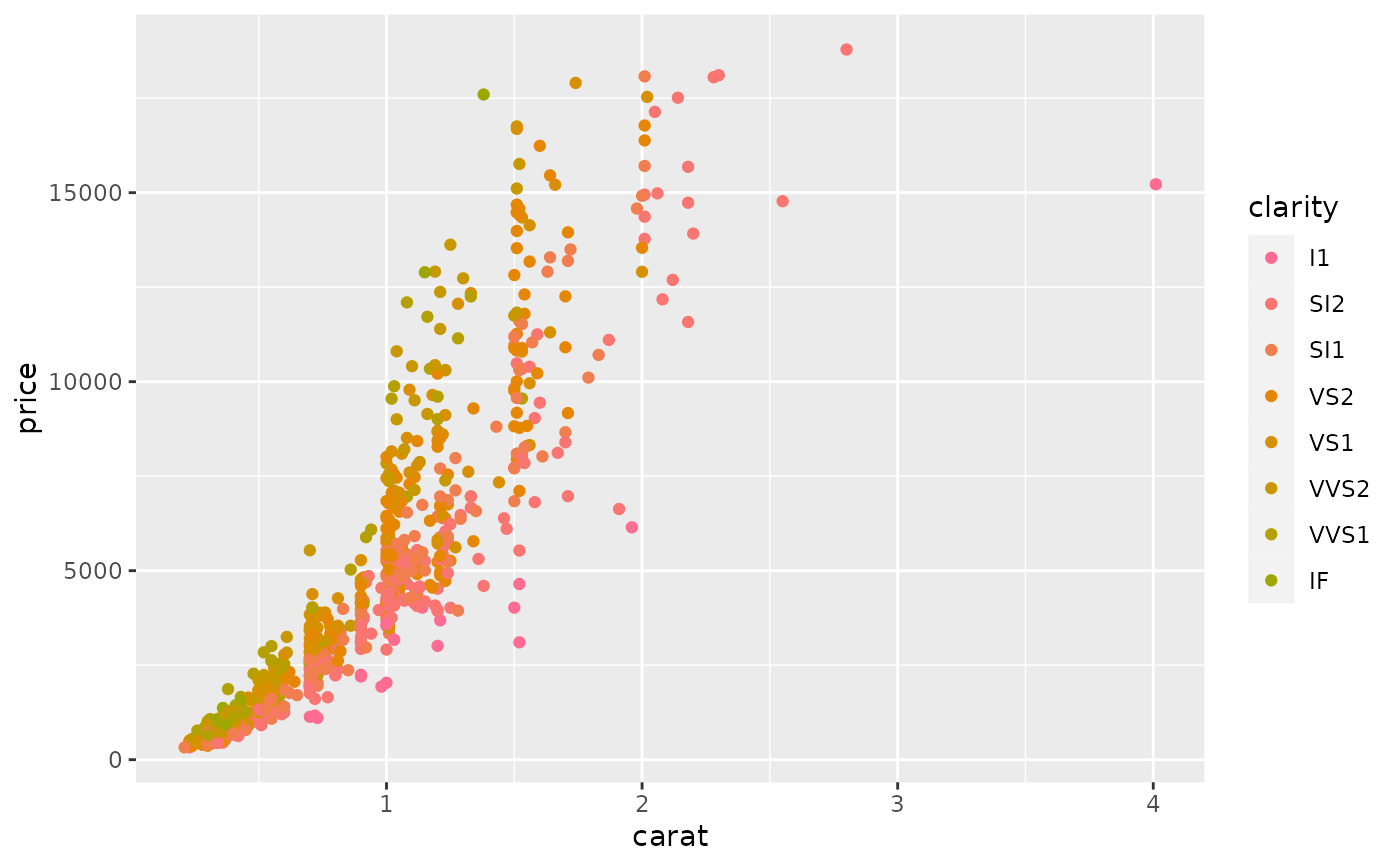
dsamp <- diamonds[sample(nrow(diamonds), 1000), ]
(d <- ggplot(dsamp, aes(carat, price)) + geom_point(aes(colour = clarity)))
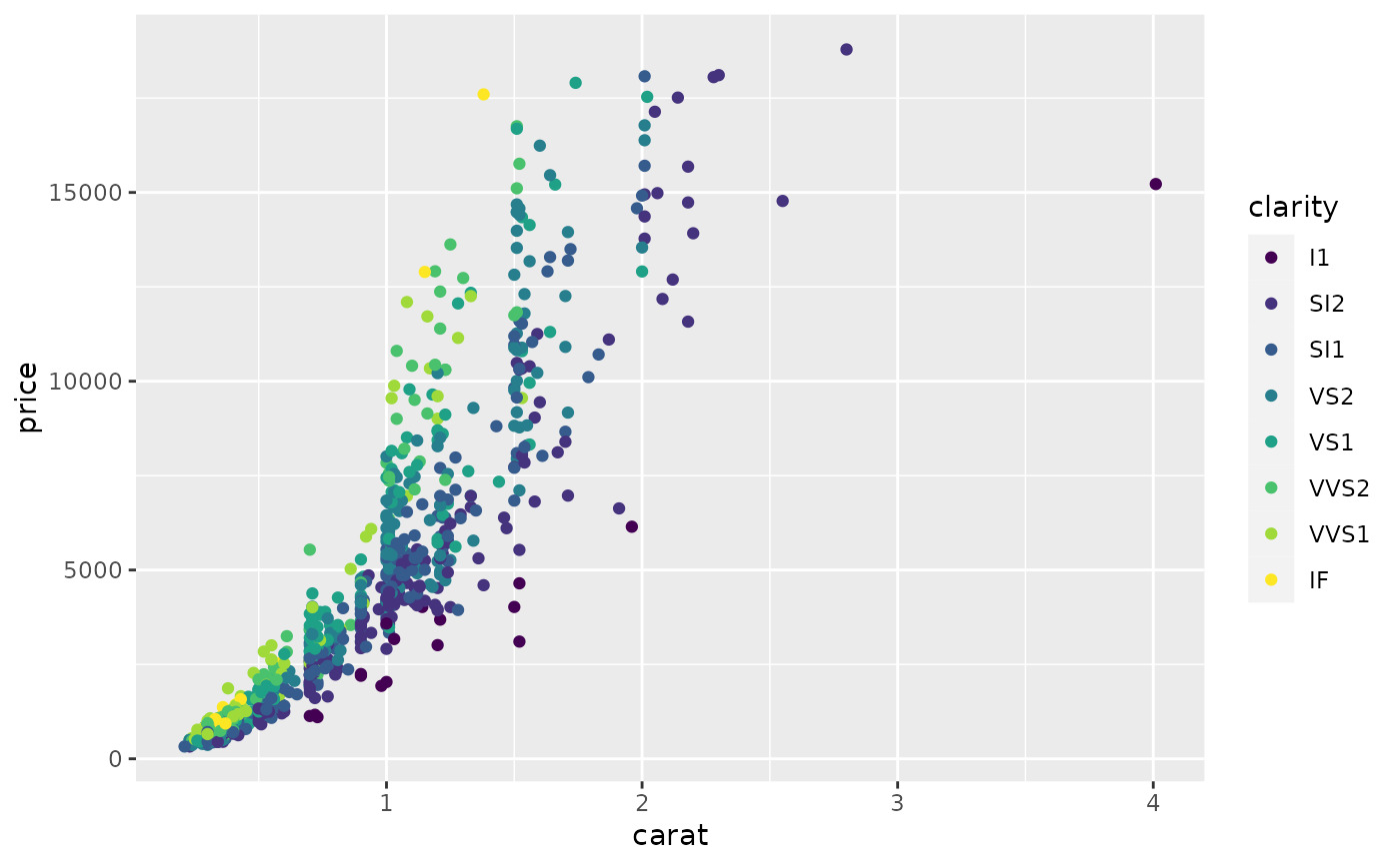 # Change scale label
d + scale_colour_hue()
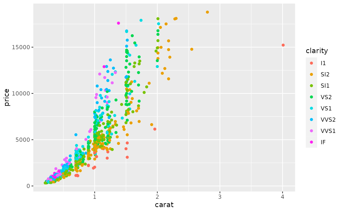
# Change scale label
d + scale_colour_hue()
 d + scale_colour_hue("clarity")
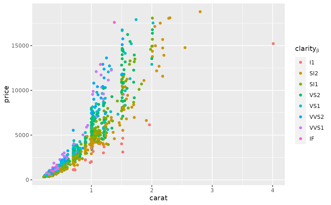
 d + scale_colour_hue(expression(clarity[beta]))
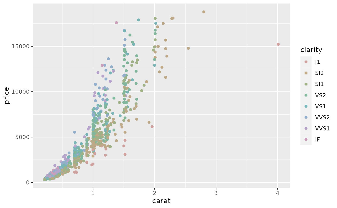
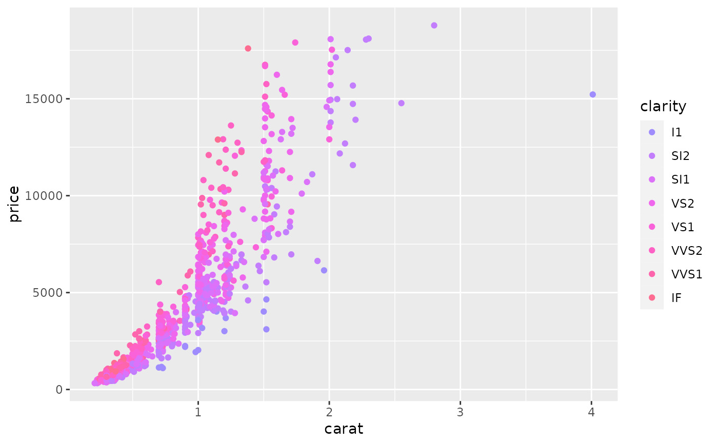
 # Adjust luminosity and chroma
d + scale_colour_hue(l = 40, c = 30)
# Adjust luminosity and chroma
d + scale_colour_hue(l = 40, c = 30)
 d + scale_colour_hue(l = 70, c = 30)
 d + scale_colour_hue(l = 70, c = 150)
 d + scale_colour_hue(l = 80, c = 150)
 # Change range of hues used
d + scale_colour_hue(h = c(0, 90))
# Change range of hues used
d + scale_colour_hue(h = c(0, 90))
 d + scale_colour_hue(h = c(90, 180))
 d + scale_colour_hue(h = c(180, 270))
 d + scale_colour_hue(h = c(270, 360))
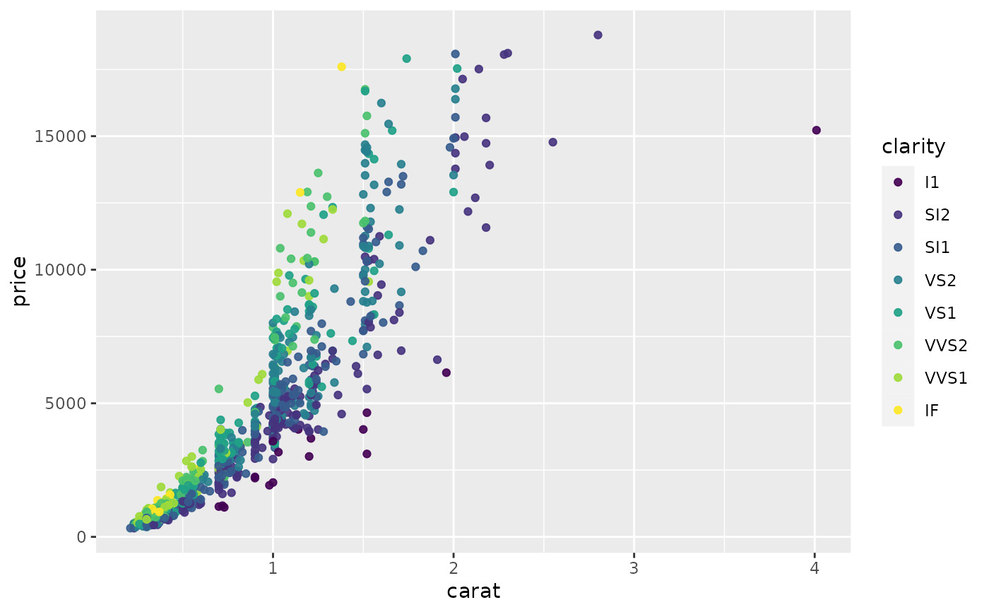
 # Vary opacity
# (only works with pdf, quartz and cairo devices)
d <- ggplot(dsamp, aes(carat, price, colour = clarity))
d + geom_point(alpha = 0.9)
# Vary opacity
# (only works with pdf, quartz and cairo devices)
d <- ggplot(dsamp, aes(carat, price, colour = clarity))
d + geom_point(alpha = 0.9)
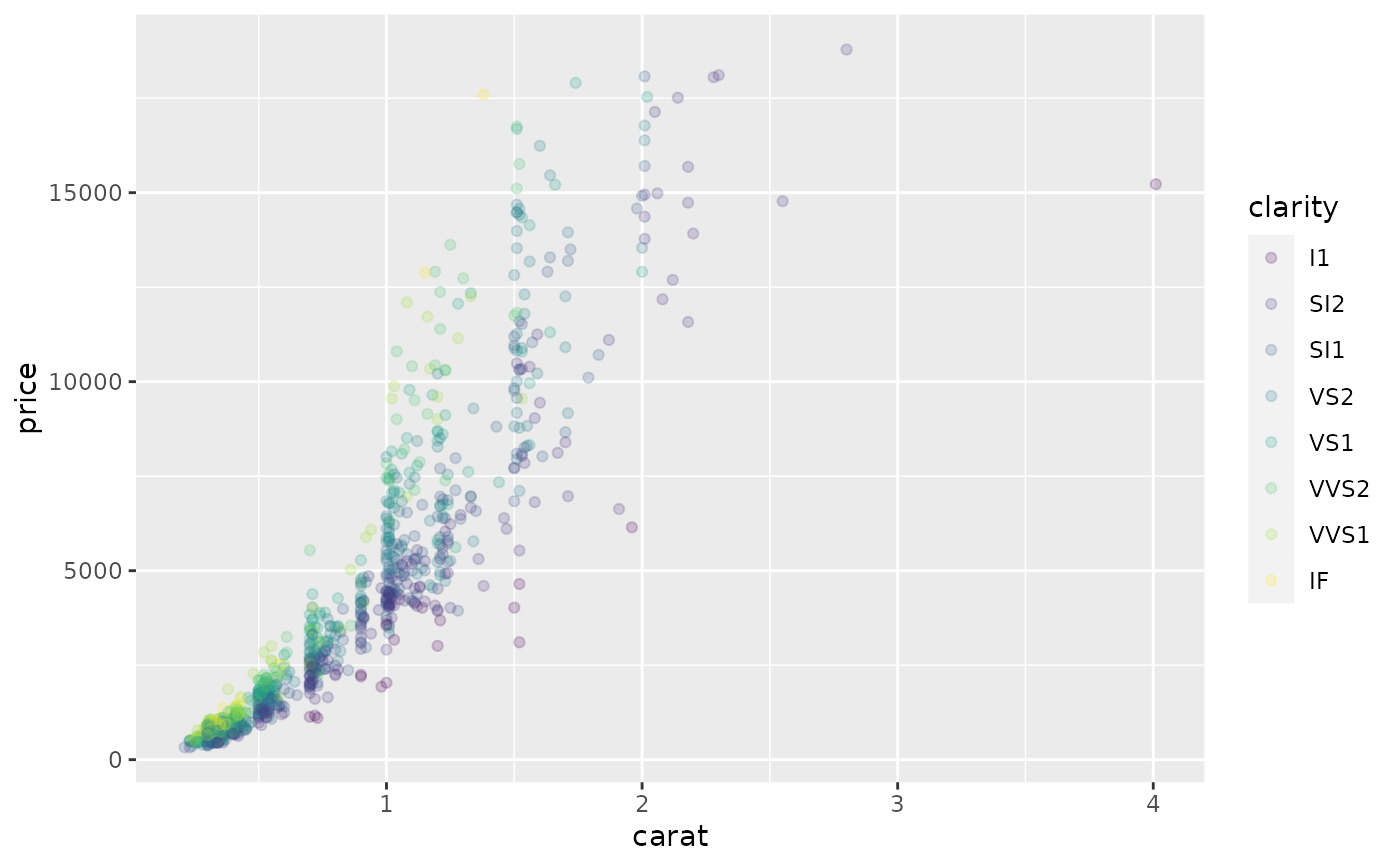
 d + geom_point(alpha = 0.5)
 d + geom_point(alpha = 0.2)
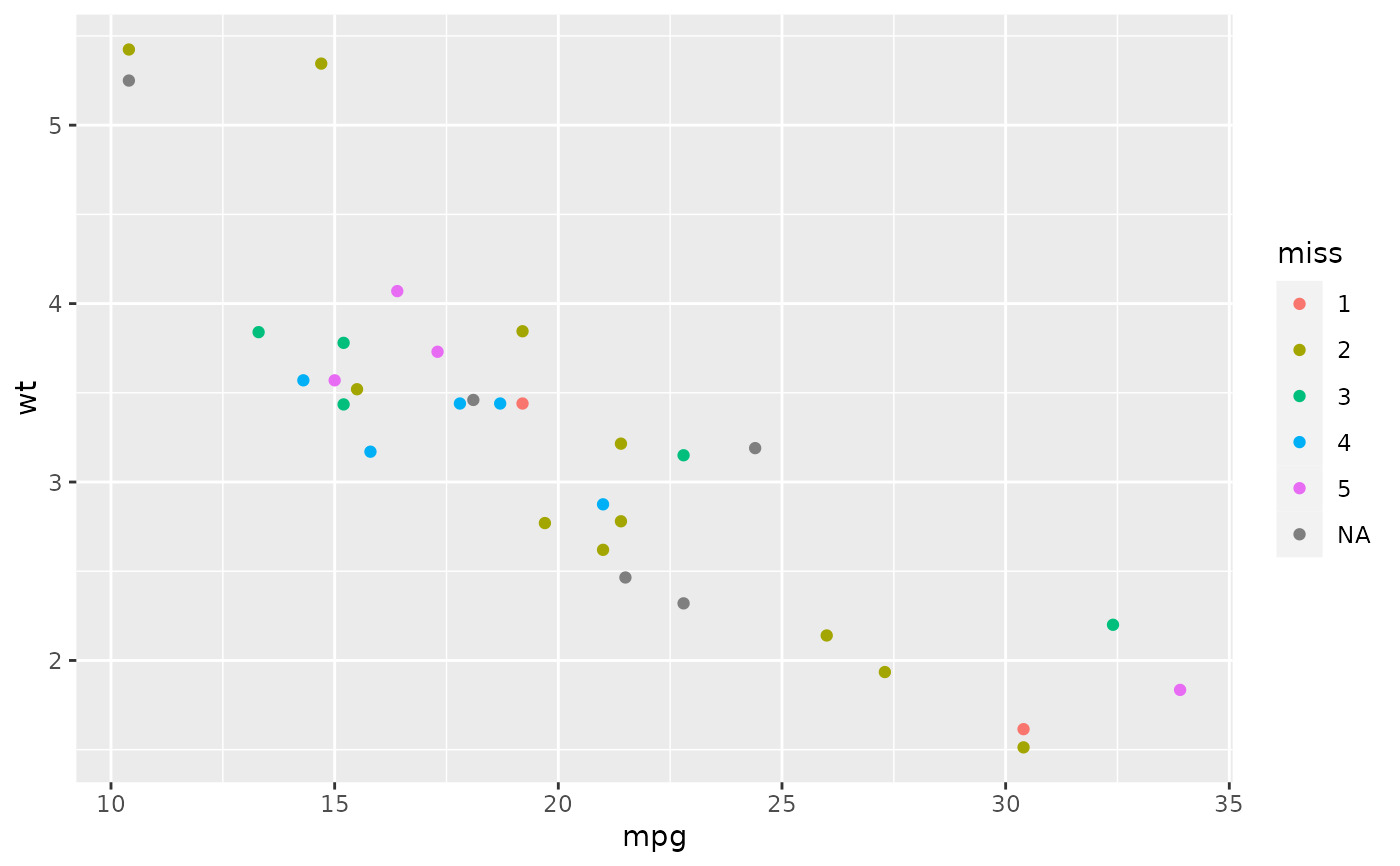
 # Colour of missing values is controlled with na.value:
miss <- factor(sample(c(NA, 1:5), nrow(mtcars), replace = TRUE))
ggplot(mtcars, aes(mpg, wt)) +
geom_point(aes(colour = miss))
# Colour of missing values is controlled with na.value:
miss <- factor(sample(c(NA, 1:5), nrow(mtcars), replace = TRUE))
ggplot(mtcars, aes(mpg, wt)) +
geom_point(aes(colour = miss))
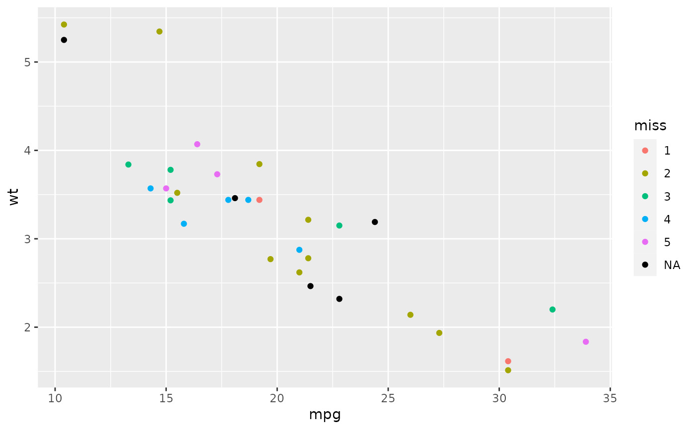
 ggplot(mtcars, aes(mpg, wt)) +
geom_point(aes(colour = miss)) +
scale_colour_hue(na.value = "black")
ggplot(mtcars, aes(mpg, wt)) +
geom_point(aes(colour = miss)) +
scale_colour_hue(na.value = "black")
 # }
# }
相关用法
- R ggplot2 scale_gradient 渐变色阶
- R ggplot2 scale_shape 形状比例,又称字形
- R ggplot2 scale_viridis 来自 viridisLite 的 Viridis 色标
- R ggplot2 scale_grey 连续灰度色阶
- R ggplot2 scale_linetype 线条图案的比例
- R ggplot2 scale_discrete 离散数据的位置尺度
- R ggplot2 scale_manual 创建您自己的离散尺度
- R ggplot2 scale_colour_discrete 离散色阶
- R ggplot2 scale_steps 分级渐变色标
- R ggplot2 scale_size 面积或半径比例
- R ggplot2 scale_date 日期/时间数据的位置刻度
- R ggplot2 scale_continuous 连续数据的位置比例(x 和 y)
- R ggplot2 scale_binned 用于对连续数据进行装箱的位置比例(x 和 y)
- R ggplot2 scale_alpha Alpha 透明度比例
- R ggplot2 scale_colour_continuous 连续色标和分级色标
- R ggplot2 scale_identity 使用不缩放的值
- R ggplot2 scale_linewidth 线宽比例
- R ggplot2 scale_brewer ColorBrewer 的连续、发散和定性色标
- R ggplot2 stat_ellipse 计算法行数据椭圆
- R ggplot2 stat_identity 保留数据原样
- R ggplot2 stat_summary_2d 以二维形式进行分类和汇总(矩形和六边形)
- R ggplot2 should_stop 在示例中用于说明何时应该发生错误。
- R ggplot2 stat_summary 总结唯一/分箱 x 处的 y 值
- R ggplot2 stat_sf_coordinates 从“sf”对象中提取坐标
- R ggplot2 stat_unique 删除重复项
注:本文由纯净天空筛选整理自Hadley Wickham等大神的英文原创作品 Evenly spaced colours for discrete data。非经特殊声明,原始代码版权归原作者所有,本译文未经允许或授权,请勿转载或复制。