R ggplot2 geom_contour 3D 表麵的 2D 輪廓

ggplot2 無法繪製真正的 3D 曲麵，但您可以使用 geom_contour() 、 geom_contour_filled() 和 geom_tile() 在 2D 中可視化 3D 曲麵。

這些函數需要常規數據，其中x 和y 坐標形成等間距網格，並且x 和y 的每個組合出現一次。允許缺失 z 值，但輪廓繪製僅適用於所有四個角均不缺失的網格點。如果您有不規則的數據，則需要在可視化之前首先使用 interp::interp() 、 akima::bilinear() 或類似工具對網格進行插值。

用法

geom_contour(
  mapping = NULL,
  data = NULL,
  stat = "contour",
  position = "identity",
  ...,
  bins = NULL,
  binwidth = NULL,
  breaks = NULL,
  lineend = "butt",
  linejoin = "round",
  linemitre = 10,
  na.rm = FALSE,
  show.legend = NA,
  inherit.aes = TRUE
)

geom_contour_filled(
  mapping = NULL,
  data = NULL,
  stat = "contour_filled",
  position = "identity",
  ...,
  bins = NULL,
  binwidth = NULL,
  breaks = NULL,
  na.rm = FALSE,
  show.legend = NA,
  inherit.aes = TRUE
)

stat_contour(
  mapping = NULL,
  data = NULL,
  geom = "contour",
  position = "identity",
  ...,
  bins = NULL,
  binwidth = NULL,
  breaks = NULL,
  na.rm = FALSE,
  show.legend = NA,
  inherit.aes = TRUE
)

stat_contour_filled(
  mapping = NULL,
  data = NULL,
  geom = "contour_filled",
  position = "identity",
  ...,
  bins = NULL,
  binwidth = NULL,
  breaks = NULL,
  na.rm = FALSE,
  show.legend = NA,
  inherit.aes = TRUE
)

參數

mapping

由 aes() 創建的一組美學映射。如果指定且inherit.aes = TRUE(默認)，它將與繪圖頂層的默認映射組合。如果沒有繪圖映射，則必須提供mapping。

data

該層要顯示的數據。有以下三種選擇：

如果默認為 NULL ，則數據繼承自 ggplot() 調用中指定的繪圖數據。

data.frame 或其他對象將覆蓋繪圖數據。所有對象都將被強化以生成 DataFrame 。請參閱fortify() 將為其創建變量。

將使用單個參數(繪圖數據)調用function。返回值必須是 data.frame ，並將用作圖層數據。可以從 formula 創建 function (例如 ~ head(.x, 10) )。

stat

用於該層數據的統計變換，可以作為 ggproto Geom 子類，也可以作為命名去掉 stat_ 前綴的統計數據的字符串(例如 "count" 而不是 "stat_count" )

position

位置調整，可以是命名調整的字符串(例如 "jitter" 使用 position_jitter )，也可以是調用位置調整函數的結果。如果需要更改調整設置，請使用後者。

...

其他參數傳遞給 layer() 。這些通常是美學，用於將美學設置為固定值，例如 colour = "red" 或 size = 3 。它們也可能是配對的 geom/stat 的參數。

bins

輪廓箱的數量。被 breaks 覆蓋。

binwidth

輪廓箱的寬度。被 bins 覆蓋。

breaks

之一：

• 用於設置輪廓中斷的數值向量

• 該函數將數據範圍和 binwidth 作為輸入，並返回中斷作為輸出。可以根據公式創建函數(例如 ~ fullseq(.x, .y))。

覆蓋 binwidth 和 bins 。默認情況下，這是一個長度為 10 且帶有 pretty() 中斷的向量。

lineend

線端樣式(圓形、對接、方形)。

linejoin

線連接樣式(圓形、斜接、斜角)。

linemitre

線斜接限製(數量大於 1)。

na.rm

如果 FALSE ，則默認缺失值將被刪除並帶有警告。如果 TRUE ，缺失值將被靜默刪除。

show.legend

合乎邏輯的。該層是否應該包含在圖例中？ NA(默認值)包括是否映射了任何美學。 FALSE 從不包含，而 TRUE 始終包含。它也可以是一個命名的邏輯向量，以精細地選擇要顯示的美學。

inherit.aes

如果 FALSE ，則覆蓋默認美學，而不是與它們組合。這對於定義數據和美觀的輔助函數最有用，並且不應繼承默認繪圖規範的行為，例如borders() 。

geom

用於顯示數據的幾何對象，可以作為 ggproto Geom 子類，也可以作為命名去除 geom_ 前綴的幾何對象的字符串(例如 "point" 而不是 "geom_point" )

美學

geom_contour() 理解以下美學(所需的美學以粗體顯示)：

• x

• y

• alpha

• colour

• group

• linetype

• linewidth

• weight

在 vignette("ggplot2-specs") 中了解有關設置這些美學的更多信息。

geom_contour_filled() 理解以下美學(所需的美學以粗體顯示)：

• x

• y

• alpha

• colour

• fill

• group

• linetype

• linewidth

• subgroup

在 vignette("ggplot2-specs") 中了解有關設置這些美學的更多信息。

stat_contour() 理解以下美學(所需的美學以粗體顯示)：

• x

• y

• z

• group

• order

在 vignette("ggplot2-specs") 中了解有關設置這些美學的更多信息。

stat_contour_filled() 理解以下美學(所需的美學以粗體顯示)：

• x

• y

• z

• fill

• group

• order

在 vignette("ggplot2-specs") 中了解有關設置這些美學的更多信息。

計算變量

這些是由層的 'stat' 部分計算的，可以使用 delayed evaluation 訪問。等高線(由 stat_contour() 計算)和等高線帶(填充輪廓，由 stat_contour_filled() 計算)的計算變量略有不同。變量 nlevel 和 piece 對兩者均可用，而 level_low 、 level_high 和 level_mid 僅適用於頻段。變量 level 是一個數字或一個因子，具體取決於是計算線還是帶。

• after_stat(level)
  輪廓高度。對於等高線，這是表示 bin 邊界的數值向量。對於等值線帶，這是表示 bin 範圍的有序因子。

• after_stat(level_low),after_stat(level_high),after_stat(level_mid)
  (僅限等值線帶)每個帶的下箱邊界和上箱邊界，以及邊界之間的中點。

• after_stat(nlevel)
  輪廓高度，最大縮放至 1。

• after_stat(piece)
  輪廓塊(整數)。

刪除變量

z

輪廓繪製後，各個數據點的 z 值不再可用。

也可以看看

例子

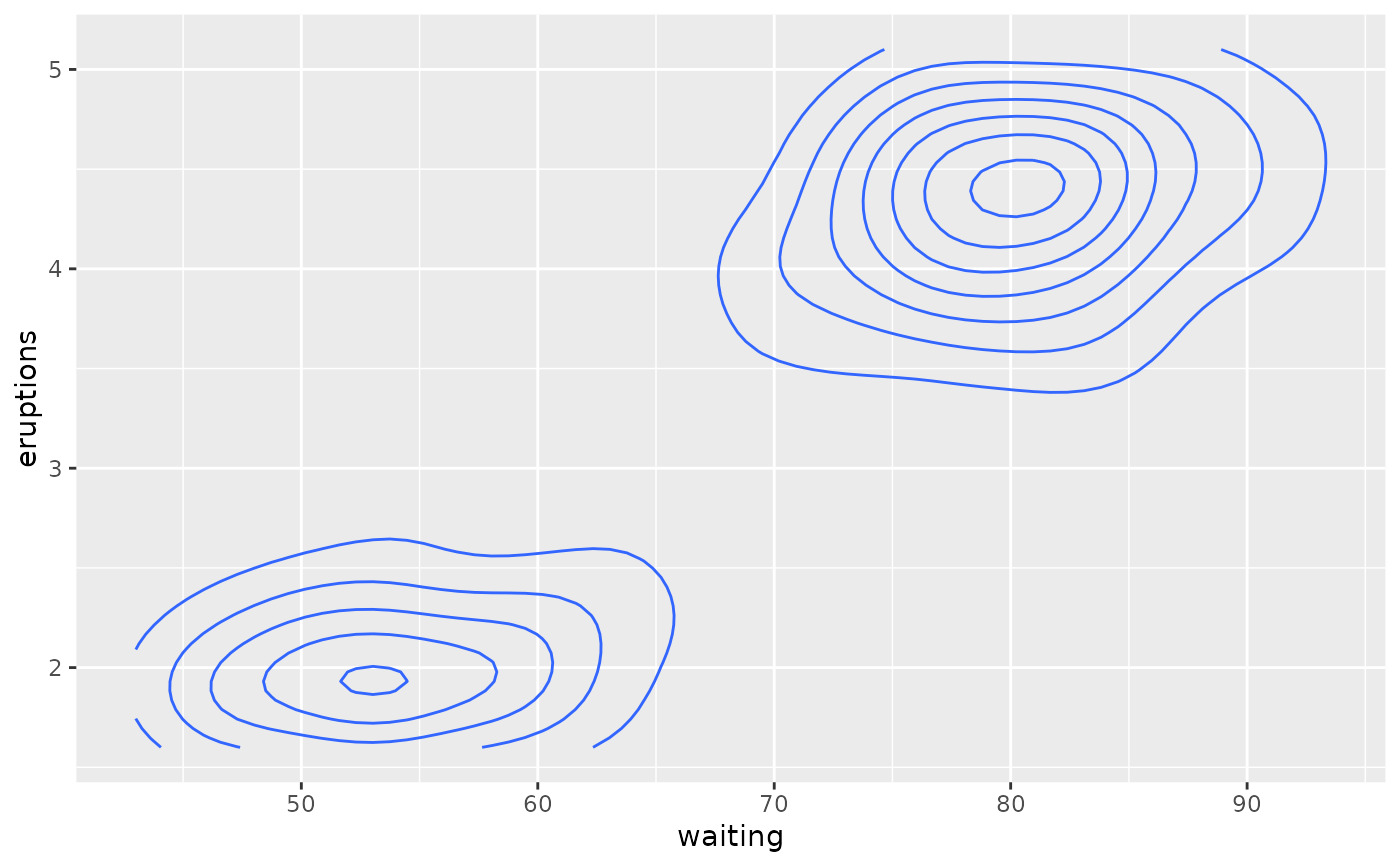
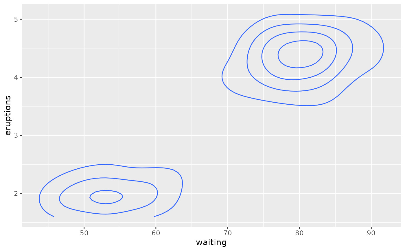
# Basic plot
v <- ggplot(faithfuld, aes(waiting, eruptions, z = density))
v + geom_contour()


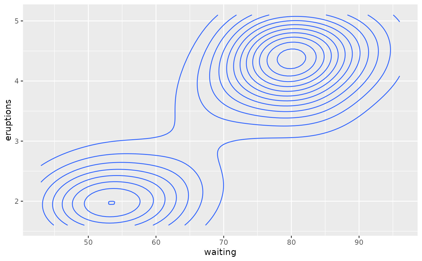
# Or compute from raw data
ggplot(faithful, aes(waiting, eruptions)) +
  geom_density_2d()


# \donttest{
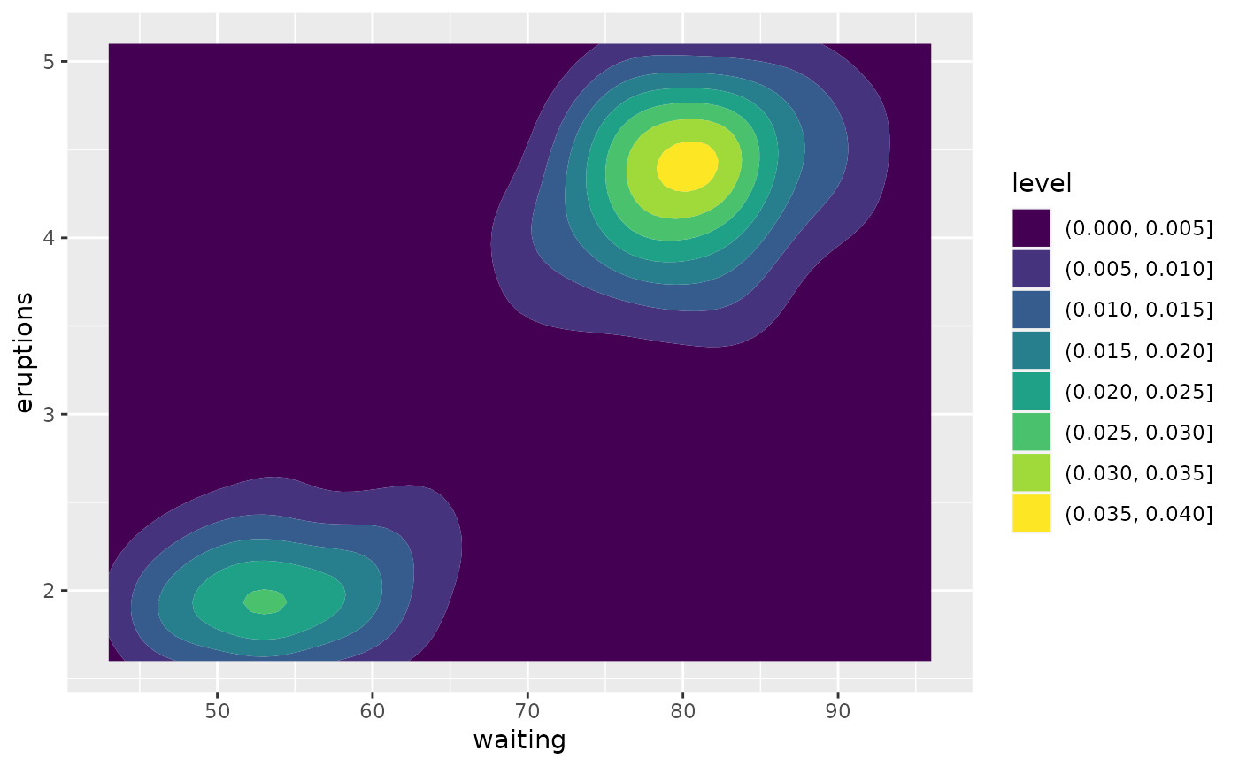
# use geom_contour_filled() for filled contours
v + geom_contour_filled()


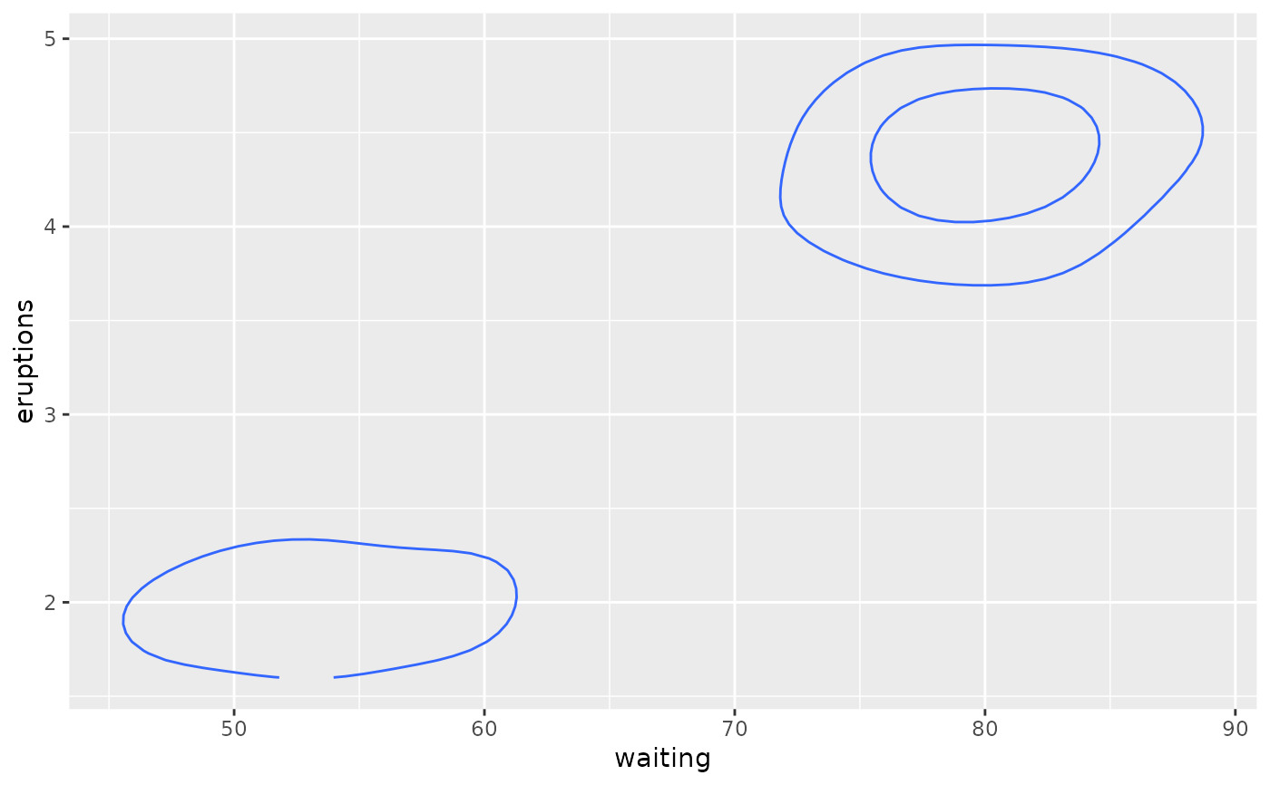
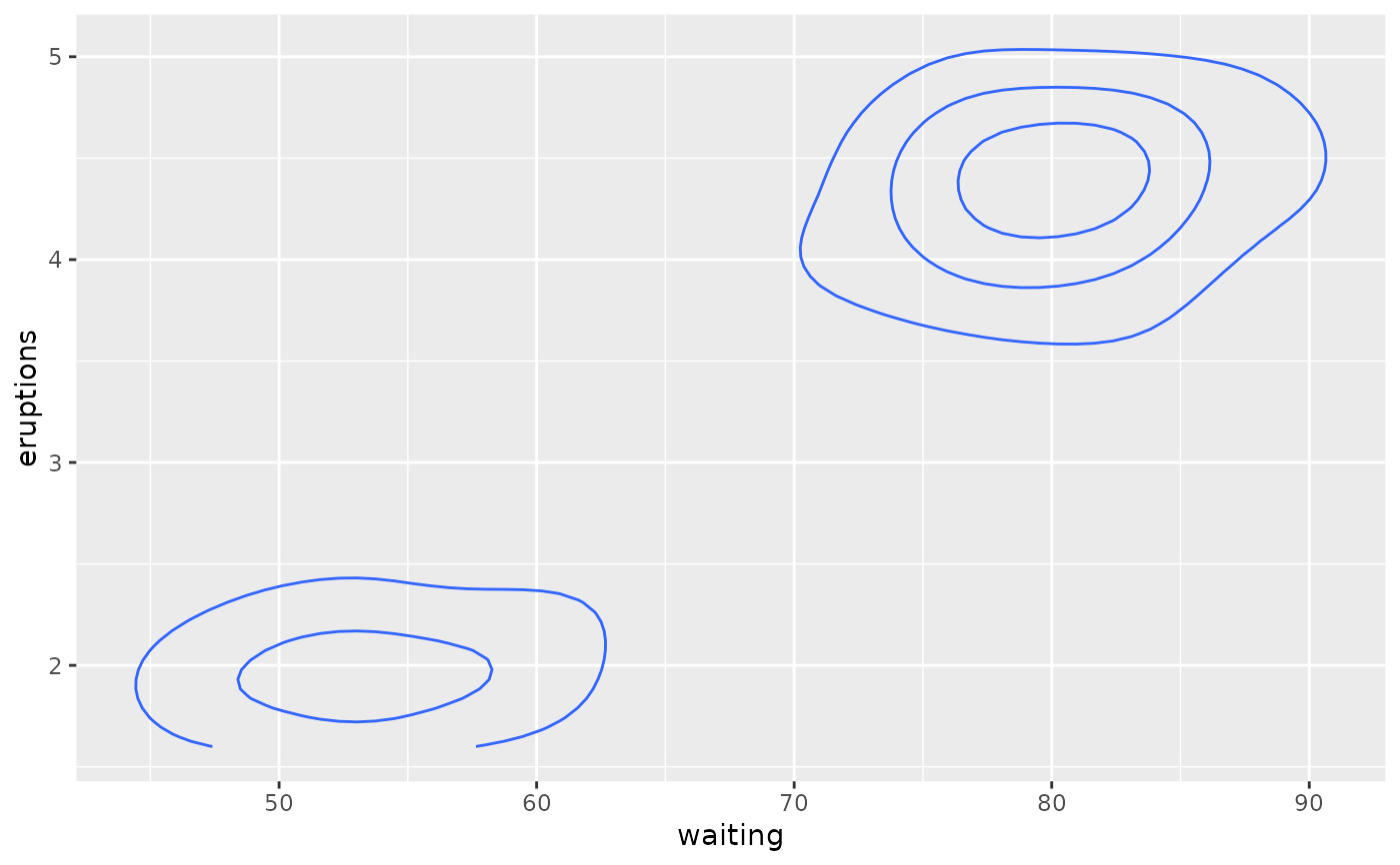
# Setting bins creates evenly spaced contours in the range of the data
v + geom_contour(bins = 3)

v + geom_contour(bins = 5)


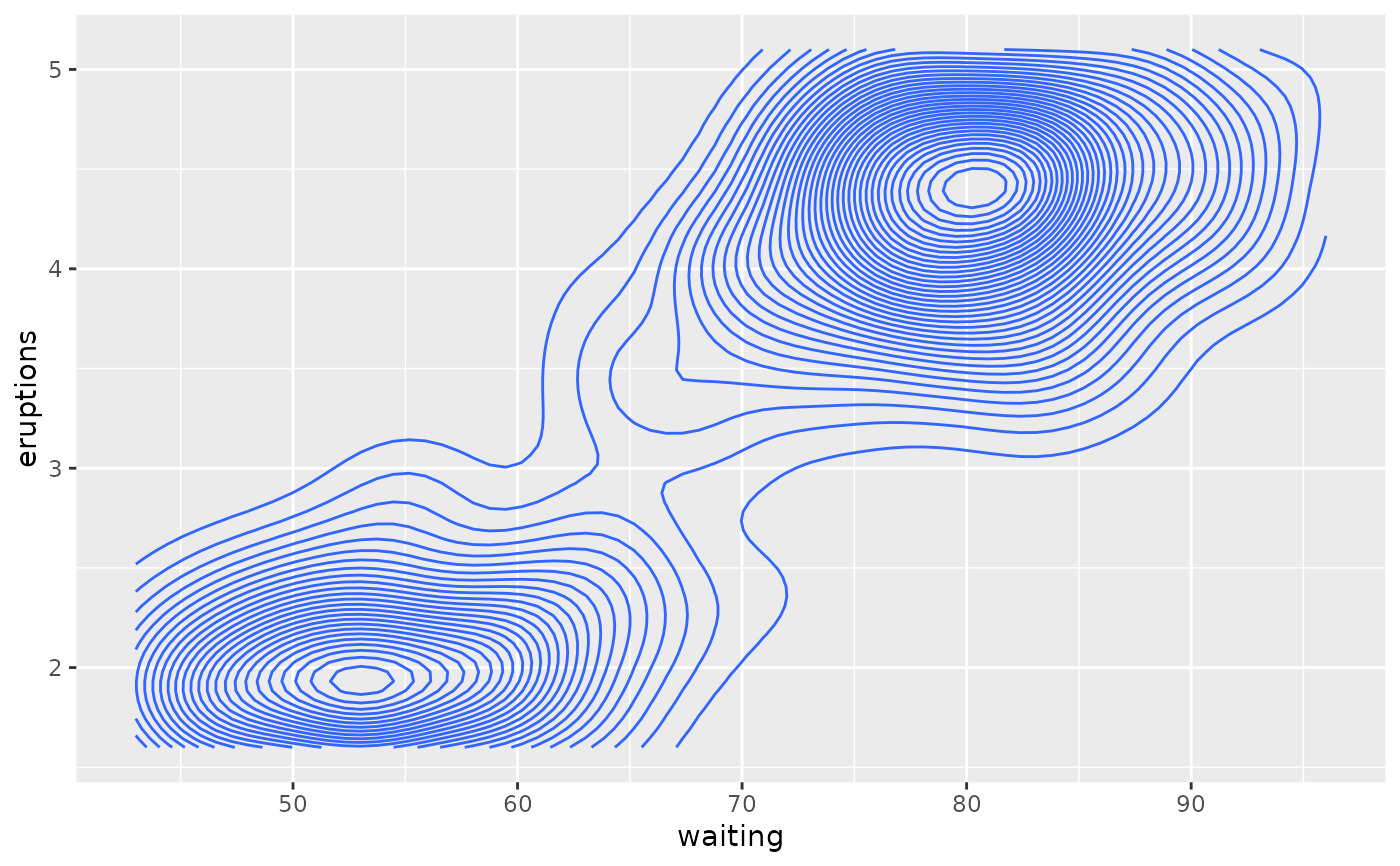
# Setting binwidth does the same thing, parameterised by the distance
# between contours
v + geom_contour(binwidth = 0.01)

v + geom_contour(binwidth = 0.001)


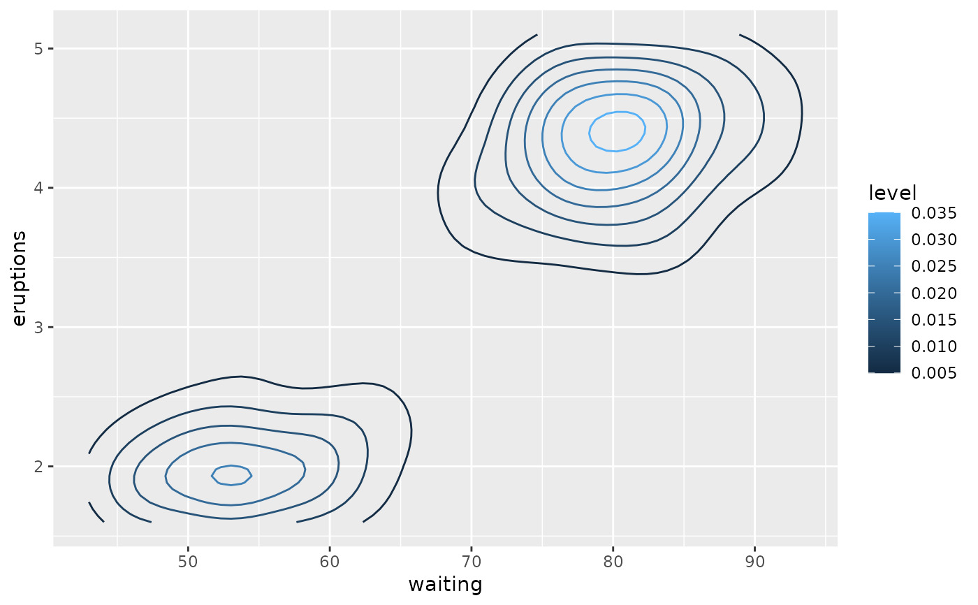
# Other parameters
v + geom_contour(aes(colour = after_stat(level)))

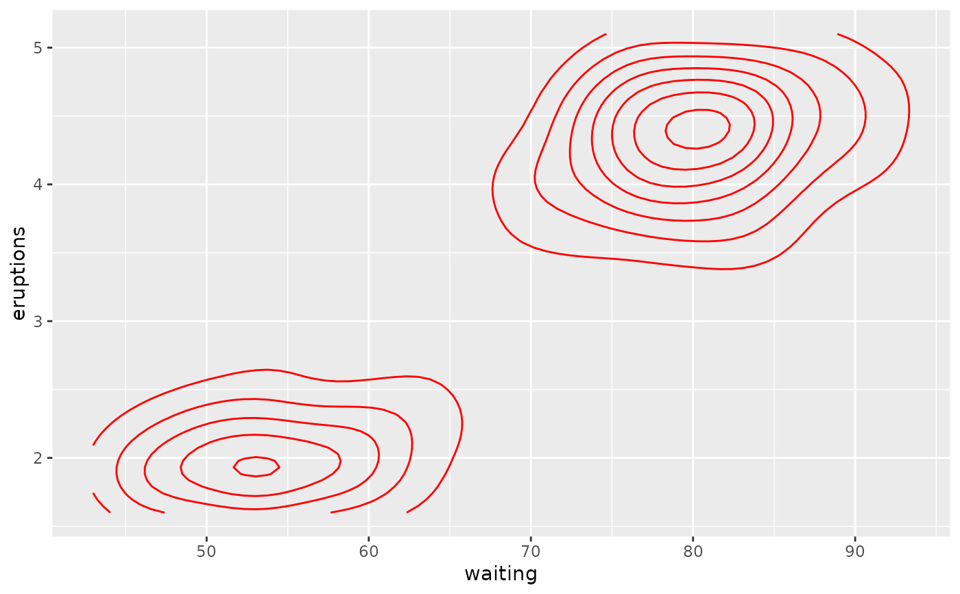
v + geom_contour(colour = "red")

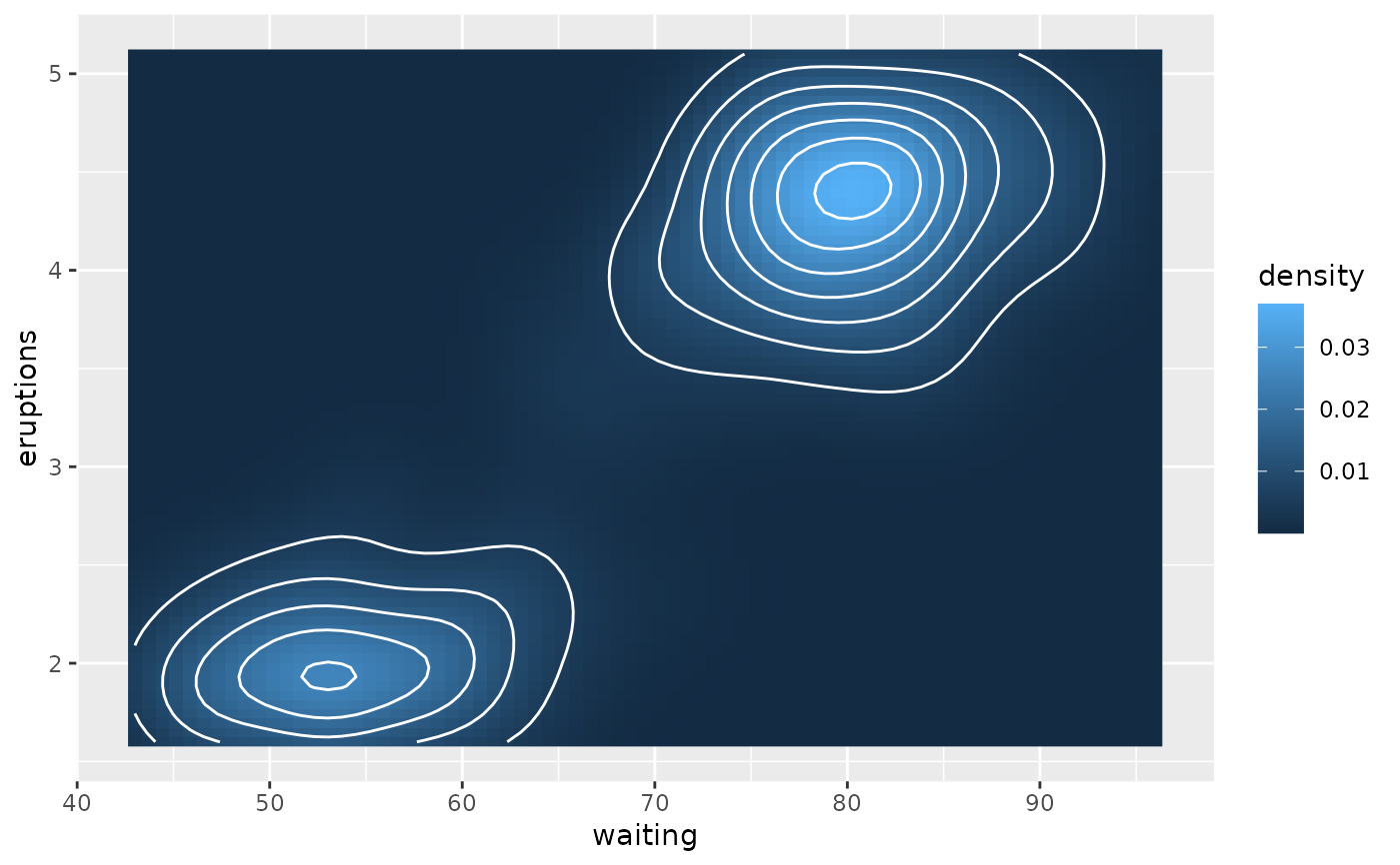
v + geom_raster(aes(fill = density)) +
  geom_contour(colour = "white")

# }