Python SciPy stats.sobol_indices用法及代碼示例

本文簡要介紹 python 語言中 scipy.stats.sobol_indices 的用法。

用法:

scipy.stats.sobol_indices(*, func, n, dists=None, method='saltelli_2010', random_state=None)#

索博爾的全局敏感性指數。

參數 ：：

func： 可調用或 dict(str, 數組)

如果 func 是可調用的函數，則用於計算 Sobol’ 索引。其簽名必須是：

func(x: ArrayLike) -> ArrayLike

形狀為 (d, n) 的 x 和形狀為 (s, n) 的輸出，其中：

• d是輸入維度函數(輸入變量的數量)，

• s是輸出維度函數(輸出變量的數量)，以及

• n是樣本數(參見n以下)。

函數評估值必須是有限的。

如果函數是一個字典，包含來自三個不同數組的函數計算。 key 必須是：f_A,f_B和f_AB.f_A和f_B應該有一個形狀(s, n)和f_AB應該有一個形狀(d, s, n)。這是一項高級函數，誤用可能會導致錯誤的分析。

n： int

用於生成矩陣的樣本數A和B。必須是 2 的冪。函數被評估將是n*(d+2).

dists： 列表(分布)，可選

每個參數的分布列表。參數的分布取決於應用，應仔細選擇。假設參數是獨立分布的，這意味著它們的值之間沒有約束或關係。

發行版必須是具有 ppf 方法的類的實例。

如果 func 是可調用的，則必須指定，否則忽略。

method： 可調用或str，默認：‘saltelli_2010’

用於計算第一個和總 Sobol 指數的方法。

如果是可調用的，其簽名必須是：

func(f_A: np.ndarray, f_B: np.ndarray, f_AB: np.ndarray)
-> Tuple[np.ndarray, np.ndarray]

形狀為 (s, n) 的 f_A, f_B 和形狀為 (d, s, n) 的 f_AB 。這些數組包含來自三組不同樣本的函數評估。輸出是形狀為 (s, d) 的第一個索引和總索引的元組。這是一項高級函數，誤用可能會導致錯誤的分析。

random_state： {無，整數， numpy.random.Generator }，可選

如果random_state是 int 或 None，一個新的numpy.random.Generator是使用創建的np.random.default_rng(random_state).如果random_state已經是一個Generator實例，然後使用提供的實例。

返回 ：：

res： SobolResult

具有屬性的對象：

first_order 形狀為 (s, d) 的 ndarray

一階 Sobol 指數。

total_order 形狀為 (s, d) 的 ndarray

總訂單 Sobol 指數。

及方法：

bootstrap(confidence_level: float, n_resamples: int) -> BootstrapSobolResult

A method providing confidence intervals on the indices. See scipy.stats.bootstrap for more details.

The bootstrapping is done on both first and total order indices, and they are available in BootstrapSobolResult as attributes first_order and total_order.

注意：

索博爾法[1],[2]是基於方差的敏感性分析，它獲得每個參數對感興趣量方差(QoIs；即輸出)的貢獻函數)。各自的貢獻可用於對參數進行排序，並通過計算模型的有效(或平均)維度來衡量模型的複雜性。

注意

假設參數是獨立分布的。每個參數仍然可以遵循任何分布。事實上，分布非常重要，應該與參數的真實分布相匹配。

它使用函數方差的函數分解來探索

\[\mathbb{V}(Y) = \sum_{i}^{d} \mathbb{V}_i (Y) + \sum_{i<j}^{d} \mathbb{V}_{ij}(Y) + ... + \mathbb{V}_{1,2,...,d}(Y),\]

引入條件方差：

\[\mathbb{V}_i(Y) = \mathbb{\mathbb{V}}[\mathbb{E}(Y|x_i)] \qquad \mathbb{V}_{ij}(Y) = \mathbb{\mathbb{V}}[\mathbb{E}(Y|x_i x_j)] - \mathbb{V}_i(Y) - \mathbb{V}_j(Y),\]

索博爾指數表示為

\[S_i = \frac{\mathbb{V}_i(Y)}{\mathbb{V}[Y]} \qquad S_{ij} =\frac{\mathbb{V}_{ij}(Y)}{\mathbb{V}[Y]}.\]

\(S_{i}\) 對應於 first-order 項，它告知 i-th 參數的貢獻，而 \(S_{ij}\) 對應於二階項，它告知 i-th 和 j-th 參數之間相互作用的貢獻。這些方程可以推廣到計算高階項；然而，它們的計算成本很高，而且它們的解釋也很複雜。這就是為什麽隻提供一階索引的原因。

總訂單指數表示參數對 QoI 方差的全局貢獻，定義為：

\[S_{T_i} = S_i + \sum_j S_{ij} + \sum_{j,k} S_{ijk} + ... = 1 - \frac{\mathbb{V}[\mathbb{E}(Y|x_{\sim i})]}{\mathbb{V}[Y]}.\]

一階指數之和至多為 1，而全階指數之和至少為 1。如果沒有交互作用，則一階指數和全階指數相等，並且一階指數和全階指數之和均為 1。

警告

負索博爾值是由於數值錯誤造成的。增加點數 n 應該會有所幫助。

進行良好分析所需的樣本數量隨著問題維度的增加而增加。例如對於 3 維問題，請考慮最小值 n >= 2**12 。模型越複雜，需要的樣本就越多。

即使對於純加性模型，由於數值噪聲，指數之和也可能不等於 1。

參考：

[1]

Sobol, I. M..“非線性數學模型的敏感性分析。”數學建模與計算實驗，1：407-414，1993。

[2]

索博爾，I.M. (2001)。 “非線性數學模型的全局敏感性指數及其蒙特卡羅估計。”模擬中的數學和計算機，55(1-3):271-280，DOI:10.1016/S0378-4754(00)00270-6，2001 年。

[3]

Saltelli, A.“充分利用模型評估來計算敏感性指數。”計算機物理通信，145(2):280-297，DOI:10.1016/S0010-4655(02)00280-1，2002 年。

[4]

Saltelli, A.、M. Ratto、T. Andres、F. Campolongo、J. Cariboni、D. Gatelli、M. Saisana 和 S. Tarantola。 “全局敏感性分析。入門書。” 2007年。

[5]

Saltelli, A.、P. Annoni、I. Azzini、F. Campolongo、M. Ratto 和 S. Tarantola。 “模型輸出的基於方差的敏感性分析。總靈敏度index的設計和估計。”計算機物理通信，181(2):259-270，DOI:10.1016/j.cpc.2009.09.018，2010。

[6]

石上，T. 和 T. Homma。 “計算機模型不確定性分析中的重要性量化技術。” IEEE，DOI:10.1109/ISUMA.1990.151285，1990。

例子：

以下是 Ishigami 函數的示例 [6]

\[Y(\mathbf{x}) = \sin x_1 + 7 \sin^2 x_2 + 0.1 x_3^4 \sin x_1,\]

與 \(\mathbf{x} \in [-\pi, \pi]^3\) 。該函數表現出很強的非線性和非單調性。

請記住，Sobol 指數假設樣本是獨立分布的。在這種情況下，我們在每個邊際上使用均勻分布。

>>> import numpy as np
>>> from scipy.stats import sobol_indices, uniform
>>> rng = np.random.default_rng()
>>> def f_ishigami(x):
...     f_eval = (
...         np.sin(x[0])
...         + 7 * np.sin(x[1])**2
...         + 0.1 * (x[2]**4) * np.sin(x[0])
...     )
...     return f_eval
>>> indices = sobol_indices(
...     func=f_ishigami, n=1024,
...     dists=[
...         uniform(loc=-np.pi, scale=2*np.pi),
...         uniform(loc=-np.pi, scale=2*np.pi),
...         uniform(loc=-np.pi, scale=2*np.pi)
...     ],
...     random_state=rng
... )
>>> indices.first_order
array([0.31637954, 0.43781162, 0.00318825])
>>> indices.total_order
array([0.56122127, 0.44287857, 0.24229595])

置信區間可以使用引導法獲得。

>>> boot = indices.bootstrap()

然後，這些信息就可以很容易地可視化。

>>> import matplotlib.pyplot as plt
>>> fig, axs = plt.subplots(1, 2, figsize=(9, 4))
>>> _ = axs[0].errorbar(
...     [1, 2, 3], indices.first_order, fmt='o',
...     yerr=[
...         indices.first_order - boot.first_order.confidence_interval.low,
...         boot.first_order.confidence_interval.high - indices.first_order
...     ],
... )
>>> axs[0].set_ylabel("First order Sobol' indices")
>>> axs[0].set_xlabel('Input parameters')
>>> axs[0].set_xticks([1, 2, 3])
>>> _ = axs[1].errorbar(
...     [1, 2, 3], indices.total_order, fmt='o',
...     yerr=[
...         indices.total_order - boot.total_order.confidence_interval.low,
...         boot.total_order.confidence_interval.high - indices.total_order
...     ],
... )
>>> axs[1].set_ylabel("Total order Sobol' indices")
>>> axs[1].set_xlabel('Input parameters')
>>> axs[1].set_xticks([1, 2, 3])
>>> plt.tight_layout()
>>> plt.show()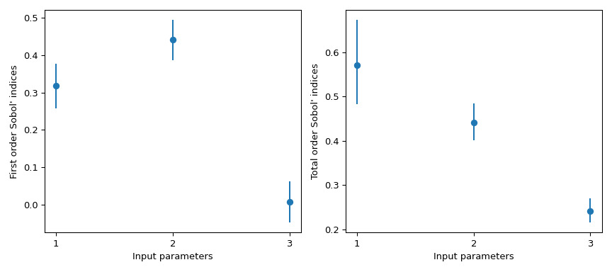

注意

默認情況下， scipy.stats.uniform 支持 [0, 1] 。使用參數 loc 和 scale ，可以獲得 [loc, loc + scale] 上的均勻分布。

這個結果特別有趣，因為一階索引 \(S_{x_3} = 0\) 而它的總順序是 \(S_{T_{x_3}} = 0.244\) 。這意味著與 \(x_3\) 的高階交互造成了差異。 QoI 上觀察到的方差中近 25% 是由於 \(x_3\) 和 \(x_1\) 之間的相關性造成的，盡管 \(x_3\) 本身對 QoI 沒有影響。

下麵給出了該函數的 Sobol 指數的直觀解釋。讓我們在 \([-\pi, \pi]^3\) 中生成 1024 個樣本並計算輸出值。

>>> from scipy.stats import qmc
>>> n_dim = 3
>>> p_labels = ['$x_1$', '$x_2$', '$x_3$']
>>> sample = qmc.Sobol(d=n_dim, seed=rng).random(1024)
>>> sample = qmc.scale(
...     sample=sample,
...     l_bounds=[-np.pi, -np.pi, -np.pi],
...     u_bounds=[np.pi, np.pi, np.pi]
... )
>>> output = f_ishigami(sample.T)

現在我們可以繪製每個參數的輸出散點圖。這提供了一種直觀的方式來了解每個參數如何影響函數的輸出。

>>> fig, ax = plt.subplots(1, n_dim, figsize=(12, 4))
>>> for i in range(n_dim):
...     xi = sample[:, i]
...     ax[i].scatter(xi, output, marker='+')
...     ax[i].set_xlabel(p_labels[i])
>>> ax[0].set_ylabel('Y')
>>> plt.tight_layout()
>>> plt.show()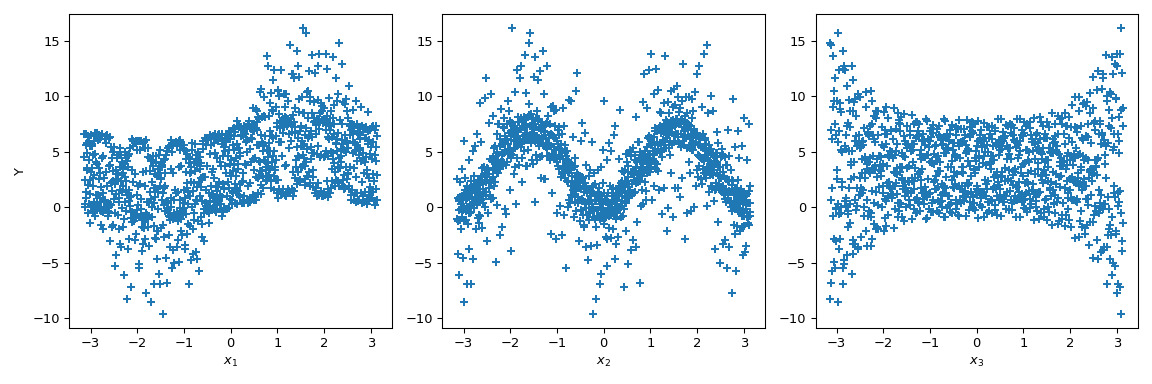

現在，Sobol' 更進一步：通過給定參數值(黑線)調節輸出值，計算條件輸出平均值。它對應於術語 \(\mathbb{E}(Y|x_i)\) 。取此項的方差即可得出 Sobol 指數的分子。

>>> mini = np.min(output)
>>> maxi = np.max(output)
>>> n_bins = 10
>>> bins = np.linspace(-np.pi, np.pi, num=n_bins, endpoint=False)
>>> dx = bins[1] - bins[0]
>>> fig, ax = plt.subplots(1, n_dim, figsize=(12, 4))
>>> for i in range(n_dim):
...     xi = sample[:, i]
...     ax[i].scatter(xi, output, marker='+')
...     ax[i].set_xlabel(p_labels[i])
...     for bin_ in bins:
...         idx = np.where((bin_ <= xi) & (xi <= bin_ + dx))
...         xi_ = xi[idx]
...         y_ = output[idx]
...         ave_y_ = np.mean(y_)
...         ax[i].plot([bin_ + dx/2] * 2, [mini, maxi], c='k')
...         ax[i].scatter(bin_ + dx/2, ave_y_, c='r')
>>> ax[0].set_ylabel('Y')
>>> plt.tight_layout()
>>> plt.show()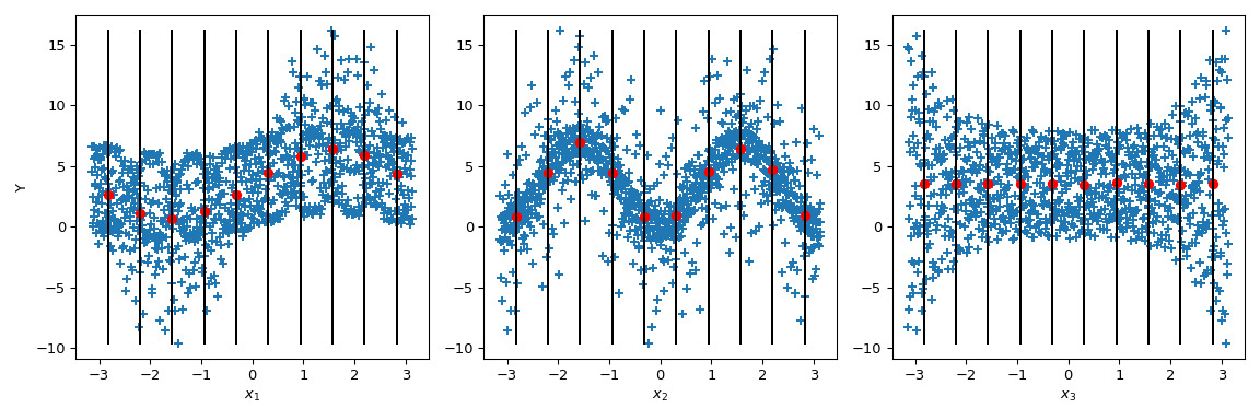

查看 \(x_3\) ，均值方差為零，導致 \(S_{x_3} = 0\) 。但我們可以進一步觀察到，輸出的方差沿著 \(x_3\) 的參數值並不是恒定的。這種異方差性可以通過高階相互作用來解釋。此外，\(x_1\) 上的異方差性也很明顯，導致 \(x_3\) 和 \(x_1\) 之間發生交互。在 \(x_2\) 上，方差似乎是恒定的，因此可以假設與此參數的交互為零。

這個案例從視覺上分析起來相當簡單——盡管它隻是定性分析。然而，當輸入參數的數量增加時，這種分析變得不現實，因為很難根據高階項得出結論。因此使用 Sobol 指數的好處。