本文簡要介紹 python 語言中 scipy.special.huber 的用法。
用法:
scipy.special.huber(delta, r, out=None) = <ufunc 'huber'>#胡貝爾損失函數。
- delta: ndarray
輸入數組,指示二次損耗與線性損耗變化點。
- r: ndarray
輸入數組,可能表示殘差。
- out: ndarray,可選
函數值的可選輸出數組
- 標量或 ndarray
計算的 Huber 損失函數值。
參數 ::
返回 ::
注意:
huber作為魯棒統計或機器學習中的損失函數,與常見的平方誤差損失相比,可減少異常值的影響,殘差的幅度高於三角洲不是平方的[1].通常,r表示殘差,即模型預測與數據之間的差異。那麽,對於,
huber類似於平方誤差並且對於絕對誤差。這樣,Huber 損失通常可以在像平方誤差損失函數這樣的小殘差模型擬合中實現快速收斂,並且仍然減少異常值的影響()就像絕對誤差損失一樣。作為是平方誤差範圍和絕對誤差範圍之間的分界線,必須針對每個問題仔細調整。huber也是凸的,使其適合基於梯度的優化。參考:
[1]彼得·胡貝爾. “位置參數的穩健估計”,1964 年。統計年鑒。 53(1):73-101。
例子:
導入所有必需的模塊。
>>> import numpy as np
>>> from scipy.special import huber
>>> import matplotlib.pyplot as plt
計算
r=2處delta=1的函數>>> huber(1., 2.) 1.5通過提供增量的 NumPy 數組或列表來計算不同增量的函數。
>>> huber([1., 3., 5.], 4.)
array([3.5, 7.5, 8. ])
通過為 r 提供 NumPy 數組或列表來計算不同點的函數。
>>> huber(2., np.array([1., 1.5, 3.]))
array([0.5  , 1.125, 4.   ])
通過為廣播提供兼容形狀的數組,可以針對不同的 delta 和 r 計算該函數。
>>> r = np.array([1., 2.5, 8., 10.])
>>> deltas = np.array([[1.], [5.], [9.]])
>>> print(r.shape, deltas.shape)
(4,) (3, 1)
>>> huber(deltas, r) array([[ 0.5 , 2. , 7.5 , 9.5 ], [ 0.5 , 3.125, 27.5 , 37.5 ], [ 0.5 , 3.125, 32. , 49.5 ]])繪製不同 delta 的函數。
>>> x = np.linspace(-4, 4, 500)
>>> deltas = [1, 2, 3]
>>> linestyles = ["dashed", "dotted", "dashdot"]
>>> fig, ax = plt.subplots()
>>> combined_plot_parameters = list(zip(deltas, linestyles))
>>> for delta, style in combined_plot_parameters:
...     ax.plot(x, huber(delta, x), label=f"$\delta={delta}$", ls=style)
>>> ax.legend(loc="upper center")
>>> ax.set_xlabel("$x$")
>>> ax.set_title("Huber loss function $h_{\delta}(x)$")
>>> ax.set_xlim(-4, 4)
>>> ax.set_ylim(0, 8)
>>> plt.show()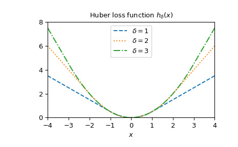
相關用法
- Python SciPy special.h1vp用法及代碼示例
- Python SciPy special.hankel1e用法及代碼示例
- Python SciPy special.hankel2e用法及代碼示例
- Python SciPy special.hyp1f1用法及代碼示例
- Python SciPy special.hyp2f1用法及代碼示例
- Python SciPy special.h2vp用法及代碼示例
- Python SciPy special.hyperu用法及代碼示例
- Python SciPy special.hyp0f1用法及代碼示例
- Python SciPy special.hermite用法及代碼示例
- Python SciPy special.exp1用法及代碼示例
- Python SciPy special.expn用法及代碼示例
- Python SciPy special.ncfdtri用法及代碼示例
- Python SciPy special.gamma用法及代碼示例
- Python SciPy special.y1用法及代碼示例
- Python SciPy special.y0用法及代碼示例
- Python SciPy special.ellip_harm_2用法及代碼示例
- Python SciPy special.i1e用法及代碼示例
- Python SciPy special.smirnovi用法及代碼示例
- Python SciPy special.ker用法及代碼示例
- Python SciPy special.ynp_zeros用法及代碼示例
- Python SciPy special.k0e用法及代碼示例
- Python SciPy special.j1用法及代碼示例
- Python SciPy special.logsumexp用法及代碼示例
- Python SciPy special.expit用法及代碼示例
- Python SciPy special.polygamma用法及代碼示例
注:本文由純淨天空篩選整理自scipy.org大神的英文原創作品 scipy.special.huber。非經特殊聲明,原始代碼版權歸原作者所有,本譯文未經允許或授權,請勿轉載或複製。