本文简要介绍 python 语言中 scipy.stats.cumfreq 的用法。
用法:
scipy.stats.cumfreq(a, numbins=10, defaultreallimits=None, weights=None)#使用 histogram 函数返回累积频率直方图。
累积直方图是一种映射,它计算所有 bin 中的累积观测数,直到指定 bin。
- a: array_like
输入数组。
- numbins: 整数,可选
用于直方图的 bin 数量。默认值为 10。
- defaultreallimits: 元组(下,上),可选
直方图范围的下限值和上限值。如果没有给出值,则范围略大于中的值的范围a用来。具体来说
(a.min() - s, a.max() + s),其中s = (1/2)(a.max() - a.min()) / (numbins - 1).- weights: 数组,可选
a中每个值的权重。默认为无,它为每个值赋予 1.0 的权重
- cumcount: ndarray
累积频率的分箱值。
- lowerlimit: 浮点数
实际下限
- binsize: 浮点数
每个 bin 的宽度。
- extrapoints: int
加分。
参数 ::
返回 ::
例子:
>>> import numpy as np
>>> import matplotlib.pyplot as plt
>>> from scipy import stats
>>> rng = np.random.default_rng()
>>> x = [1, 4, 2, 1, 3, 1]
>>> res = stats.cumfreq(x, numbins=4, defaultreallimits=(1.5, 5))
>>> res.cumcount
array([ 1.,  2.,  3.,  3.])
>>> res.extrapoints
3
创建具有 1000 个随机值的正态分布
>>> samples = stats.norm.rvs(size=1000, random_state=rng)计算累积频率
>>> res = stats.cumfreq(samples, numbins=25)计算 x 的值空间
>>> x = res.lowerlimit + np.linspace(0, res.binsize*res.cumcount.size,
...                                  res.cumcount.size)
绘制直方图和累积直方图
>>> fig = plt.figure(figsize=(10, 4))
>>> ax1 = fig.add_subplot(1, 2, 1)
>>> ax2 = fig.add_subplot(1, 2, 2)
>>> ax1.hist(samples, bins=25)
>>> ax1.set_title('Histogram')
>>> ax2.bar(x, res.cumcount, width=res.binsize)
>>> ax2.set_title('Cumulative histogram')
>>> ax2.set_xlim([x.min(), x.max()])
>>> plt.show()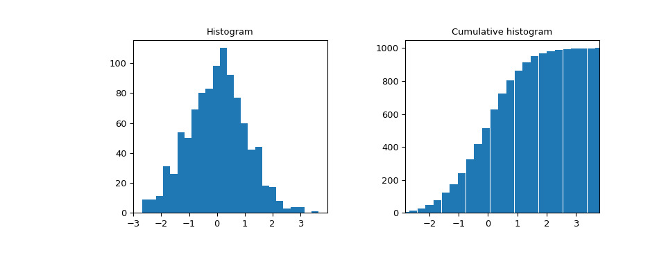
相关用法
- Python SciPy stats.cosine用法及代码示例
- Python SciPy stats.chisquare用法及代码示例
- Python SciPy stats.chi2用法及代码示例
- Python SciPy stats.circmean用法及代码示例
- Python SciPy stats.chi用法及代码示例
- Python SciPy stats.cramervonmises用法及代码示例
- Python SciPy stats.cauchy用法及代码示例
- Python SciPy stats.circvar用法及代码示例
- Python SciPy stats.combine_pvalues用法及代码示例
- Python SciPy stats.circstd用法及代码示例
- Python SciPy stats.crystalball用法及代码示例
- Python SciPy stats.chi2_contingency用法及代码示例
- Python SciPy stats.cramervonmises_2samp用法及代码示例
- Python SciPy stats.anderson用法及代码示例
- Python SciPy stats.iqr用法及代码示例
- Python SciPy stats.genpareto用法及代码示例
- Python SciPy stats.skewnorm用法及代码示例
- Python SciPy stats.norminvgauss用法及代码示例
- Python SciPy stats.directional_stats用法及代码示例
- Python SciPy stats.invwishart用法及代码示例
- Python SciPy stats.bartlett用法及代码示例
- Python SciPy stats.levy_stable用法及代码示例
- Python SciPy stats.page_trend_test用法及代码示例
- Python SciPy stats.itemfreq用法及代码示例
- Python SciPy stats.exponpow用法及代码示例
注:本文由纯净天空筛选整理自scipy.org大神的英文原创作品 scipy.stats.cumfreq。非经特殊声明,原始代码版权归原作者所有,本译文未经允许或授权,请勿转载或复制。