Python SciPy stats.bootstrap用法及代码示例

本文简要介绍 python 语言中 scipy.stats.bootstrap 的用法。

用法:

scipy.stats.bootstrap(data, statistic, *, n_resamples=9999, batch=None, vectorized=None, paired=False, axis=0, confidence_level=0.95, alternative='two-sided', method='BCa', bootstrap_result=None, random_state=None)#

计算统计量的两侧引导置信区间。

什么时候方法是'percentile'和选择是'two-sided'，根据以下过程计算自举置信区间。

1. 对数据重新采样：对于data中的每个样本和n_resamples中的每一个，随机抽取与原始样本大小相同的原始样本(有放回)。

2. 计算统计量的引导分布：对于每组重采样，计算检验统计量。

3. 确定置信区间：找到自举分布的区间，即

   • 对称于中位数和

   • 包含confidence_level 个重采样统计值。

虽然 'percentile' 方法最直观，但在实践中很少使用。有两种更常见的方法可用，'basic'(“反向百分位数”)和'BCa'(“偏差校正和加速”)；它们的不同之处在于步骤 3 的执行方式。

如果样本在数据从它们各自的分布中随机抽取\(n\)次，置信区间返回bootstrap将包含这些分布的统计数据的真实值confidence_level\(\, \times \, n\)次。

参数 ：：

data： 类似数组的序列

每个数据元素都是来自底层分布的样本。

statistic： 可调用的

要计算置信区间的统计量。统计必须是接受的可调用对象len(data)样本作为单独的参数并返回结果统计信息。如果矢量化已设置True,统计还必须接受关键字参数轴并被矢量化以计算沿提供的统计量轴.

n_resamples： 整数，默认值：9999

为形成统计量的自举分布而执行的重采样次数。

batch： 整数，可选

在每个向量化调用中要处理的重采样数统计.内存使用量为 O(批*n)， 在哪里n是样本量。默认为None， 在这种情况下batch = n_resamples(或者batch = max(n_resamples, n)为了method='BCa')。

vectorized： 布尔型，可选

如果矢量化已设置False,统计不会传递关键字参数轴并且预计仅计算一维样本的统计量。如果True,统计将传递关键字参数轴并预计将计算统计数据轴当传递 ND 样本数组时。如果None(默认)，矢量化将被设置True如果axis是一个参数统计。使用矢量化统计通常可以减少计算时间。

paired： 布尔值，默认值：False

统计数据是否将数据中样本的对应元素视为配对。

axis： 整数，默认值：0

沿其计算统计量的数据中样本的轴。

confidence_level： 浮点数，默认：0.95

置信区间的置信水平。

alternative： {‘双面’,‘less’, ‘greater’}，默认：'two-sided'

选择'two-sided'(默认)对于双边置信区间，'less'对于单边置信区间，下限为-np.inf， 和'greater'对于单边置信区间，其上限为np.inf。单边置信区间的另一个界限与双边置信区间的相同confidence_level距离 1.0 相差两倍；例如95% 的上限'less'置信区间与 90% 的上限相同'two-sided'置信区间。

method： {‘percentile’, ‘basic’, ‘bca’}，默认：'BCa'

是否返回 ‘percentile’ 引导置信区间 ( 'percentile' )、‘basic’ (AKA ‘reverse’) 引导置信区间 ( 'basic' ) 或偏差校正和加速引导置信区间 ( 'BCa' ) 。

bootstrap_result： BootstrapResult，可选

提供先前调用返回的结果对象bootstrap将以前的 bootstrap 发行版包含在新的 bootstrap 发行版中。例如，这可以用来改变confidence_level， 改变方法，或者查看执行额外重采样而不重复计算的效果。

random_state： {无，整数， numpy.random.Generator ，

numpy.random.RandomState}, optional

用于生成重采样的伪随机数生成器状态。

如果random_state是None(或者np.random)， 这numpy.random.RandomState使用单例。如果random_state是一个 int，一个新的RandomState使用实例，播种random_state.如果random_state已经是一个Generator或者RandomState实例然后使用该实例。

返回 ：：

res： BootstrapResult

具有属性的对象：

confidence_interval ConfidenceInterval

引导置信区间作为一个实例collections.namedtuple有属性低的和高的.

bootstrap_distribution ndarray

自举分布，即统计对于每次重新采样。最后一个维度与重新采样相对应(例如res.bootstrap_distribution.shape[-1] == n_resamples)。

standard_error 浮点数或 ndarray

Bootstrap 标准误，即 Bootstrap 分布的样本标准差。

警告 ：：

DegenerateDataWarning

当 method='BCa' 且引导分布退化时生成(例如，所有元素都相同)。

注意：

置信区间的元素可能是NaNmethod='BCa'如果引导分布是退化的(例如所有元素都是相同的)。在这种情况下，考虑使用另一个方法或检查数据以表明其他分析可能更合适(例如，所有观察结果都是相同的)。

参考：

[1]

B. Efron 和 R. J. Tibshirani，Bootstrap 简介，Chapman & Hall/CRC，博卡拉顿，佛罗里达州，美国(1993 年)

[2]

Nathaniel E. Helwig，“Bootstrap Confidence Intervals”，http://users.stat.umn.edu/~helwig/notes/bootci-Notes.pdf

[3]

自举(统计)，维基百科，https://en.wikipedia.org/wiki/Bootstrapping_%28statistics%29

例子：

假设我们从未知分布中采样数据。

>>> import numpy as np
>>> rng = np.random.default_rng()
>>> from scipy.stats import norm
>>> dist = norm(loc=2, scale=4)  # our "unknown" distribution
>>> data = dist.rvs(size=100, random_state=rng)

我们对分布的标准差感兴趣。

>>> std_true = dist.std()      # the true value of the statistic
>>> print(std_true)
4.0
>>> std_sample = np.std(data)  # the sample statistic
>>> print(std_sample)
3.9460644295563863

如果我们要从未知分布中重复采样并每次计算样本的统计量，则引导程序用于近似我们期望的变异性。它通过替换地重复对原始样本的值进行重采样并计算每个重采样的统计量来实现此目的。这会产生“bootstrap distribution” 统计数据。

>>> import matplotlib.pyplot as plt
>>> from scipy.stats import bootstrap
>>> data = (data,)  # samples must be in a sequence
>>> res = bootstrap(data, np.std, confidence_level=0.9,
...                 random_state=rng)
>>> fig, ax = plt.subplots()
>>> ax.hist(res.bootstrap_distribution, bins=25)
>>> ax.set_title('Bootstrap Distribution')
>>> ax.set_xlabel('statistic value')
>>> ax.set_ylabel('frequency')
>>> plt.show()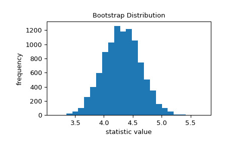

标准误差量化了这种变异性。它被计算为引导分布的标准差。

>>> res.standard_error
0.24427002125829136
>>> res.standard_error == np.std(res.bootstrap_distribution, ddof=1)
True

统计量的自举分布通常近似正态，其尺度等于标准误差。

>>> x = np.linspace(3, 5)
>>> pdf = norm.pdf(x, loc=std_sample, scale=res.standard_error)
>>> fig, ax = plt.subplots()
>>> ax.hist(res.bootstrap_distribution, bins=25, density=True)
>>> ax.plot(x, pdf)
>>> ax.set_title('Normal Approximation of the Bootstrap Distribution')
>>> ax.set_xlabel('statistic value')
>>> ax.set_ylabel('pdf')
>>> plt.show()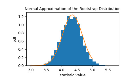

这表明我们可以根据该正态分布的分位数构建统计量的 90% 置信区间。

>>> norm.interval(0.9, loc=std_sample, scale=res.standard_error)
(3.5442759991341726, 4.3478528599786)

由于中心极限定理，这种正态近似对于样本背后的各种统计数据和分布都是准确的；然而，该近似值并非在所有情况下都可靠。由于 bootstrap 旨在处理任意基础分布和统计数据，因此它使用更先进的技术来生成准确的置信区间。

>>> print(res.confidence_interval)
ConfidenceInterval(low=3.57655333533867, high=4.382043696342881)

如果我们从原始分布中采样 1000 次并为每个样本形成引导置信区间，则置信区间大约 90% 的时间包含统计量的真实值。

>>> n_trials = 1000
>>> ci_contains_true_std = 0
>>> for i in range(n_trials):
...    data = (dist.rvs(size=100, random_state=rng),)
...    ci = bootstrap(data, np.std, confidence_level=0.9, n_resamples=1000,
...                   random_state=rng).confidence_interval
...    if ci[0] < std_true < ci[1]:
...        ci_contains_true_std += 1
>>> print(ci_contains_true_std)
875

除了编写循环之外，我们还可以一次确定所有 1000 个样本的置信区间。

>>> data = (dist.rvs(size=(n_trials, 100), random_state=rng),)
>>> res = bootstrap(data, np.std, axis=-1, confidence_level=0.9,
...                 n_resamples=1000, random_state=rng)
>>> ci_l, ci_u = res.confidence_interval

这里，ci_l和ci_u包含每个的置信区间n_trials = 1000样品。

>>> print(ci_l[995:])
[3.77729695 3.75090233 3.45829131 3.34078217 3.48072829]
>>> print(ci_u[995:])
[4.88316666 4.86924034 4.32032996 4.2822427  4.59360598]

同样，大约 90% 包含真实值 std_true = 4 。

>>> print(np.sum((ci_l < std_true) & (std_true < ci_u)))
900

bootstrap也可用于估计多样本统计的置信区间，包括通过假设检验计算的置信区间。scipy.stats.mood执行等尺度参数的 Mood 检验，它返回两个输出：统计量和 p 值。为了获得检验统计量的置信区间，我们首先换行scipy.stats.mood在接受两个样本参数的函数中，接受一个轴关键字参数，并仅返回统计信息。

>>> from scipy.stats import mood
>>> def my_statistic(sample1, sample2, axis):
...     statistic, _ = mood(sample1, sample2, axis=-1)
...     return statistic

在这里，我们使用具有默认 95% 置信水平的 ‘percentile’ 方法。

>>> sample1 = norm.rvs(scale=1, size=100, random_state=rng)
>>> sample2 = norm.rvs(scale=2, size=100, random_state=rng)
>>> data = (sample1, sample2)
>>> res = bootstrap(data, my_statistic, method='basic', random_state=rng)
>>> print(mood(sample1, sample2)[0])  # element 0 is the statistic
-5.521109549096542
>>> print(res.confidence_interval)
ConfidenceInterval(low=-7.255994487314675, high=-4.016202624747605)

标准误差的 bootstrap 估计也是可用的。

>>> print(res.standard_error)
0.8344963846318795

配对样本统计也有效。例如，考虑 Pearson 相关系数。

>>> from scipy.stats import pearsonr
>>> n = 100
>>> x = np.linspace(0, 10, n)
>>> y = x + rng.uniform(size=n)
>>> print(pearsonr(x, y)[0])  # element 0 is the statistic
0.9962357936065914

我们包装 pearsonr 以便它只返回统计信息。

>>> def my_statistic(x, y):
...     return pearsonr(x, y)[0]

我们使用 paired=True 调用 bootstrap 。此外，由于 my_statistic 未进行矢量化以计算沿给定轴的统计量，因此我们传入 vectorized=False 。

>>> res = bootstrap((x, y), my_statistic, vectorized=False, paired=True,
...                 random_state=rng)
>>> print(res.confidence_interval)
ConfidenceInterval(low=0.9950085825848624, high=0.9971212407917498)

结果对象可以传回到bootstrap以执行额外的重采样：

>>> len(res.bootstrap_distribution)
9999
>>> res = bootstrap((x, y), my_statistic, vectorized=False, paired=True,
...                 n_resamples=1001, random_state=rng,
...                 bootstrap_result=res)
>>> len(res.bootstrap_distribution)
11000

或更改置信区间选项：

>>> res2 = bootstrap((x, y), my_statistic, vectorized=False, paired=True,
...                  n_resamples=0, random_state=rng, bootstrap_result=res,
...                  method='percentile', confidence_level=0.9)
>>> np.testing.assert_equal(res2.bootstrap_distribution,
...                         res.bootstrap_distribution)
>>> res.confidence_interval
ConfidenceInterval(low=0.9950035351407804, high=0.9971170323404578)

无需重复计算原始引导分布。