position_stack() 將條形堆疊在一起; position_fill() 堆疊條形並將每個堆疊標準化為具有恒定的高度。
參數
- vjust
-
對具有位置(如點或線)而不是尺寸(如條形或區域)的幾何圖形進行垂直調整。設置為
0以與底部對齊,0.5為中間對齊,1(默認值)為頂部對齊。 - reverse
-
如果是
TRUE,將反轉默認的堆疊順序。如果您要旋轉繪圖和圖例,這非常有用。
細節
position_fill() 和 position_stack() 自動以與組美學相反的順序堆疊值,對於條形圖來說,這通常由填充美學定義(默認組美學由除 x 和 y 之外的所有離散美學的組合形成)。此默認值可確保條形顏色與默認圖例對齊。
根據您的需要,可以通過三種方式覆蓋默認值:
-
更改基礎因子中的級別順序。這將更改堆疊順序以及圖例中鍵的順序。
-
設置圖例
breaks以更改鍵的順序而不影響堆疊。 -
手動設置組美學以更改堆疊順序而不影響圖例。
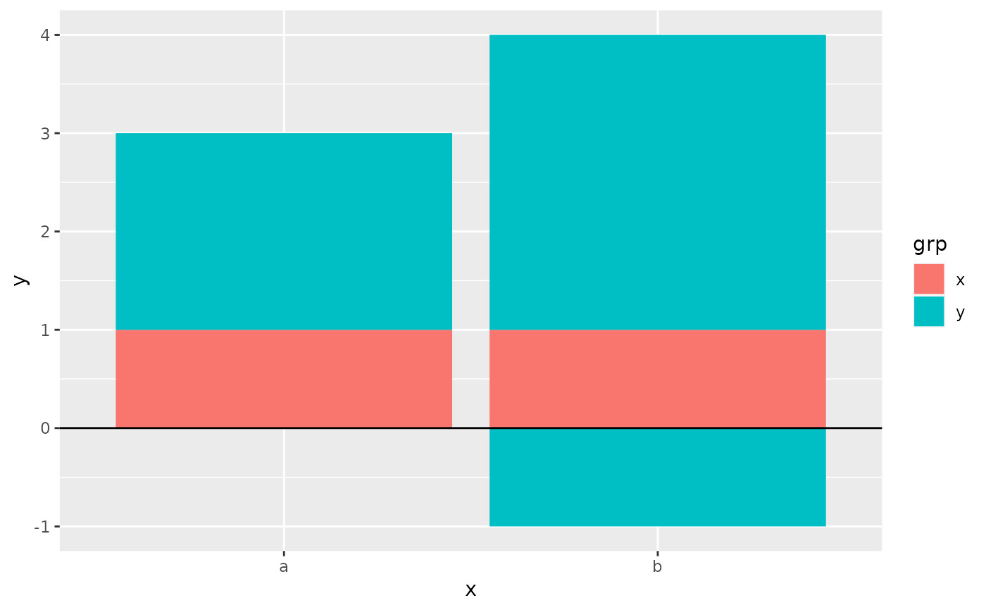
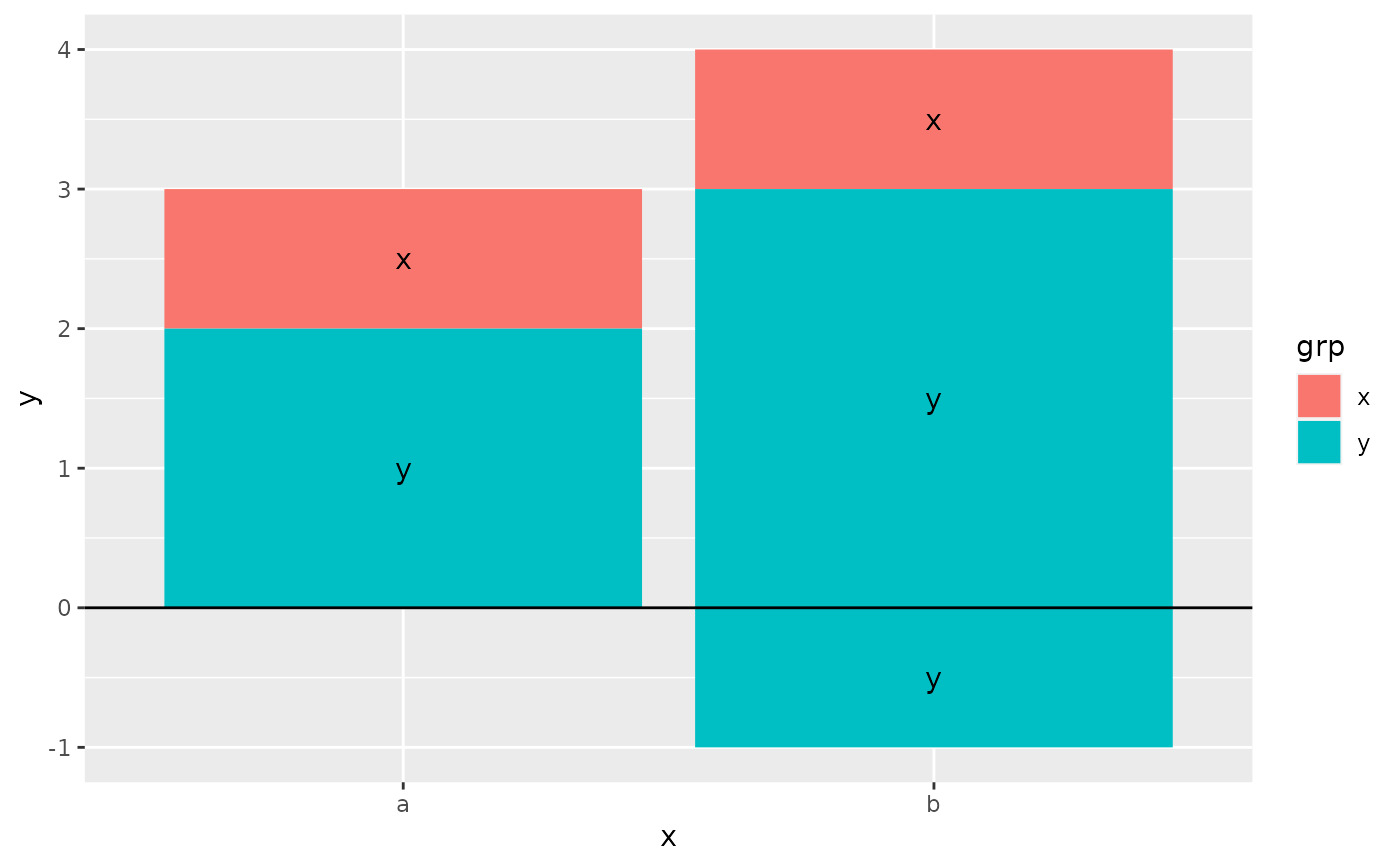
正值和負值的堆疊是單獨執行的,因此正值從 x 軸向上堆疊,負值向下堆疊。
由於堆疊是在尺度變換之後執行的,因此使用非線性尺度進行堆疊會產生扭曲,很容易導致數據的誤解。因此,不鼓勵將這些位置調整與尺度變換(例如對數或平方根尺度)結合使用。
也可以看看
有關更多示例,請參閱geom_bar() 和 geom_area()。
其他位置調整:position_dodge()、position_identity()、position_jitterdodge()、position_jitter()、position_nudge()
例子
# Stacking and filling ------------------------------------------------------
# Stacking is the default behaviour for most area plots.
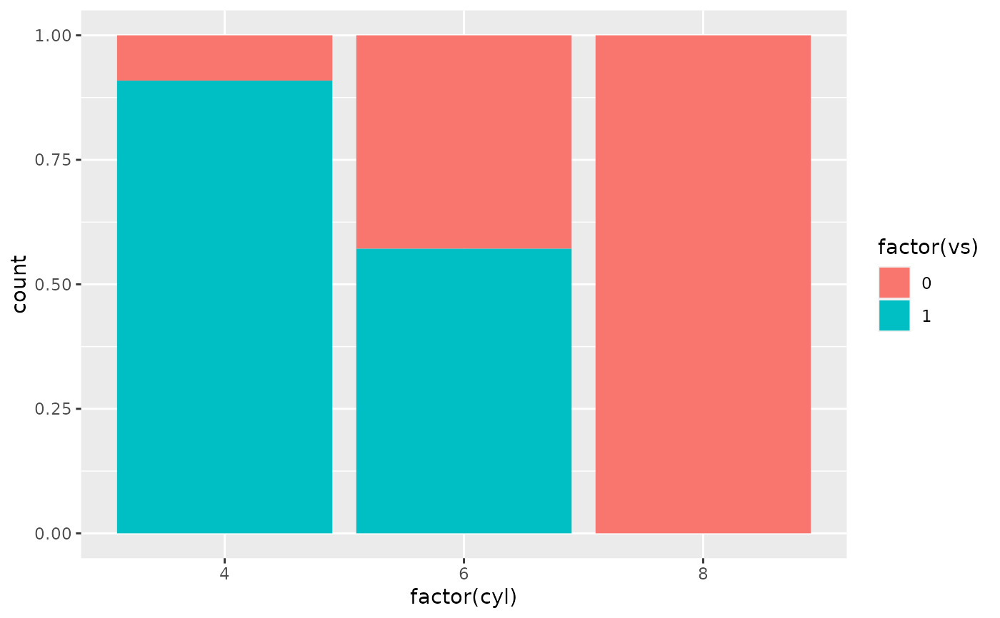
# Fill makes it easier to compare proportions
ggplot(mtcars, aes(factor(cyl), fill = factor(vs))) +
geom_bar()
 ggplot(mtcars, aes(factor(cyl), fill = factor(vs))) +
geom_bar(position = "fill")
ggplot(mtcars, aes(factor(cyl), fill = factor(vs))) +
geom_bar(position = "fill")
 ggplot(diamonds, aes(price, fill = cut)) +
geom_histogram(binwidth = 500)
ggplot(diamonds, aes(price, fill = cut)) +
geom_histogram(binwidth = 500)
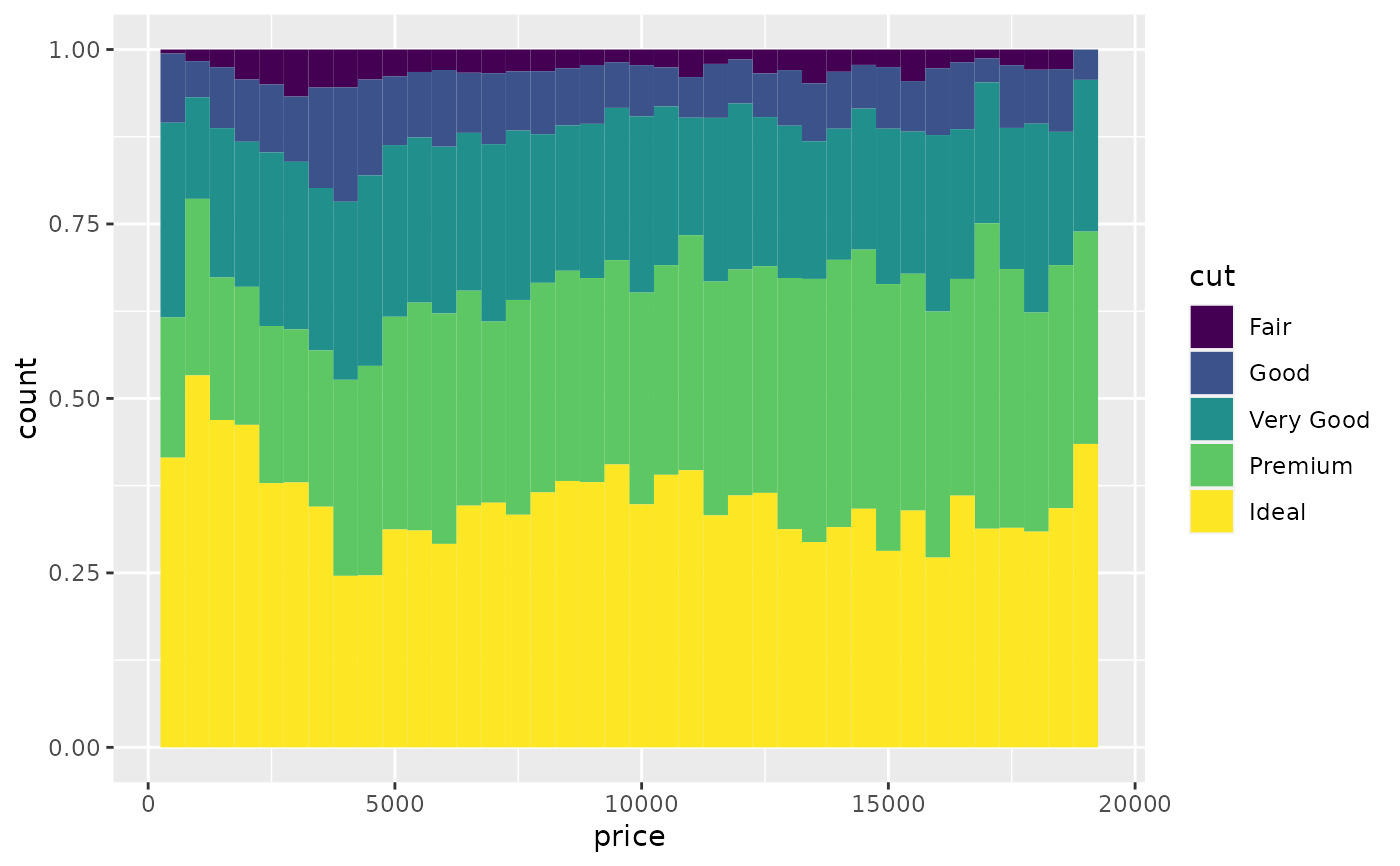
 ggplot(diamonds, aes(price, fill = cut)) +
geom_histogram(binwidth = 500, position = "fill")
ggplot(diamonds, aes(price, fill = cut)) +
geom_histogram(binwidth = 500, position = "fill")
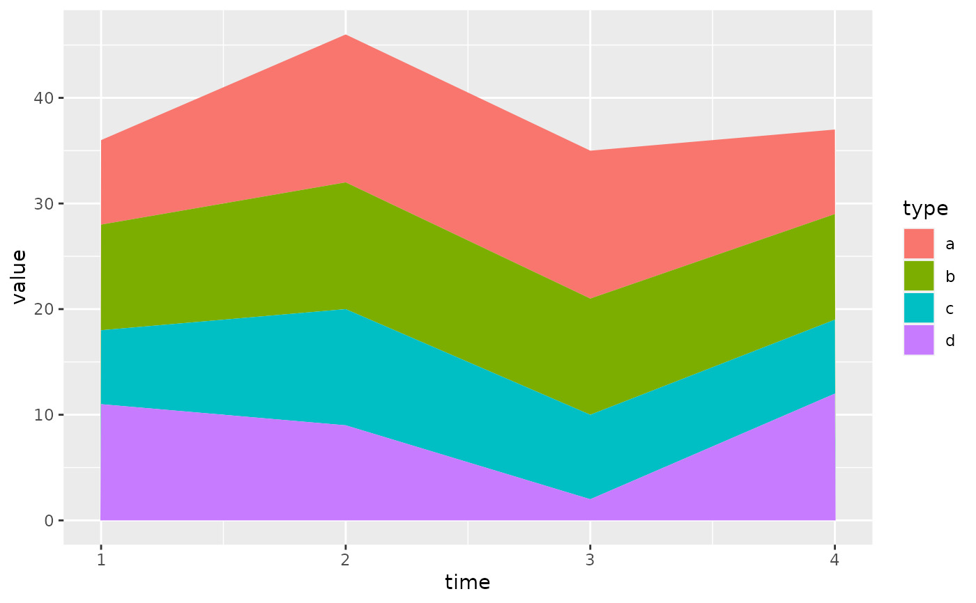
 # Stacking is also useful for time series
set.seed(1)
series <- data.frame(
time = c(rep(1, 4),rep(2, 4), rep(3, 4), rep(4, 4)),
type = rep(c('a', 'b', 'c', 'd'), 4),
value = rpois(16, 10)
)
ggplot(series, aes(time, value)) +
geom_area(aes(fill = type))
# Stacking is also useful for time series
set.seed(1)
series <- data.frame(
time = c(rep(1, 4),rep(2, 4), rep(3, 4), rep(4, 4)),
type = rep(c('a', 'b', 'c', 'd'), 4),
value = rpois(16, 10)
)
ggplot(series, aes(time, value)) +
geom_area(aes(fill = type))
 # Stacking order ------------------------------------------------------------
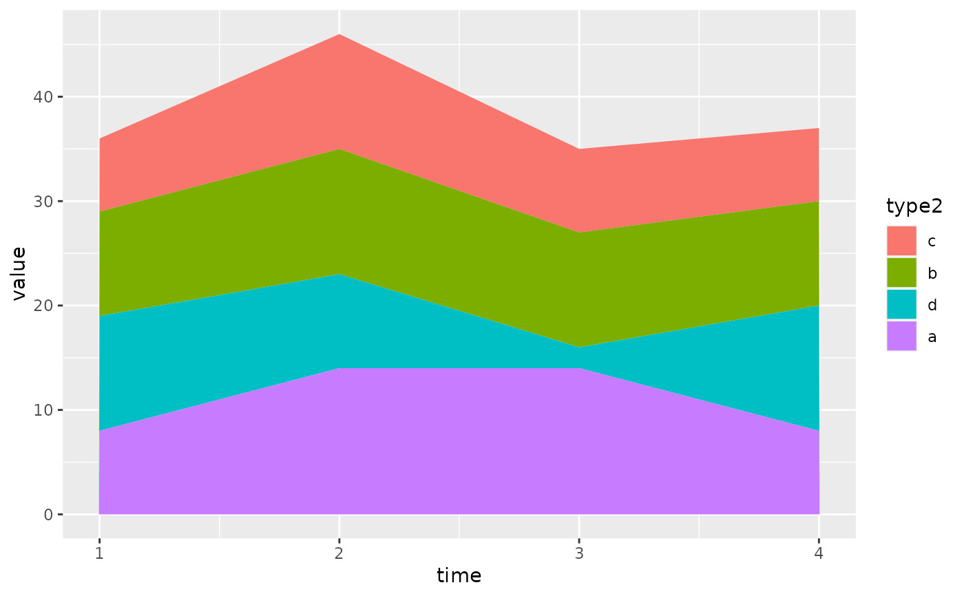
# The stacking order is carefully designed so that the plot matches
# the legend.
# You control the stacking order by setting the levels of the underlying
# factor. See the forcats package for convenient helpers.
series$type2 <- factor(series$type, levels = c('c', 'b', 'd', 'a'))
ggplot(series, aes(time, value)) +
geom_area(aes(fill = type2))
# Stacking order ------------------------------------------------------------
# The stacking order is carefully designed so that the plot matches
# the legend.
# You control the stacking order by setting the levels of the underlying
# factor. See the forcats package for convenient helpers.
series$type2 <- factor(series$type, levels = c('c', 'b', 'd', 'a'))
ggplot(series, aes(time, value)) +
geom_area(aes(fill = type2))
 # You can change the order of the levels in the legend using the scale
ggplot(series, aes(time, value)) +
geom_area(aes(fill = type)) +
scale_fill_discrete(breaks = c('a', 'b', 'c', 'd'))
# You can change the order of the levels in the legend using the scale
ggplot(series, aes(time, value)) +
geom_area(aes(fill = type)) +
scale_fill_discrete(breaks = c('a', 'b', 'c', 'd'))
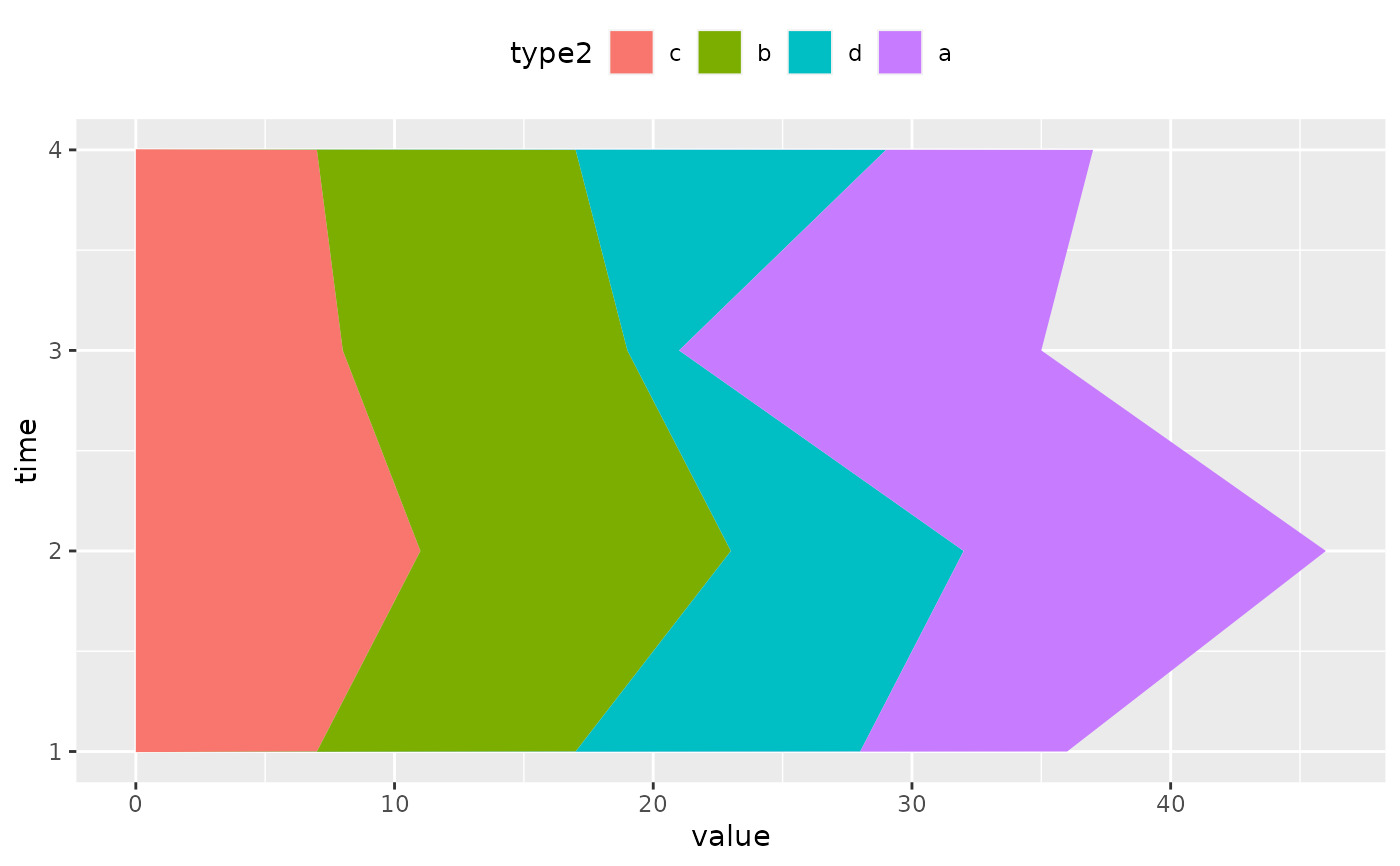
 # If you've flipped the plot, use reverse = TRUE so the levels
# continue to match
ggplot(series, aes(time, value)) +
geom_area(aes(fill = type2), position = position_stack(reverse = TRUE)) +
coord_flip() +
theme(legend.position = "top")
# If you've flipped the plot, use reverse = TRUE so the levels
# continue to match
ggplot(series, aes(time, value)) +
geom_area(aes(fill = type2), position = position_stack(reverse = TRUE)) +
coord_flip() +
theme(legend.position = "top")
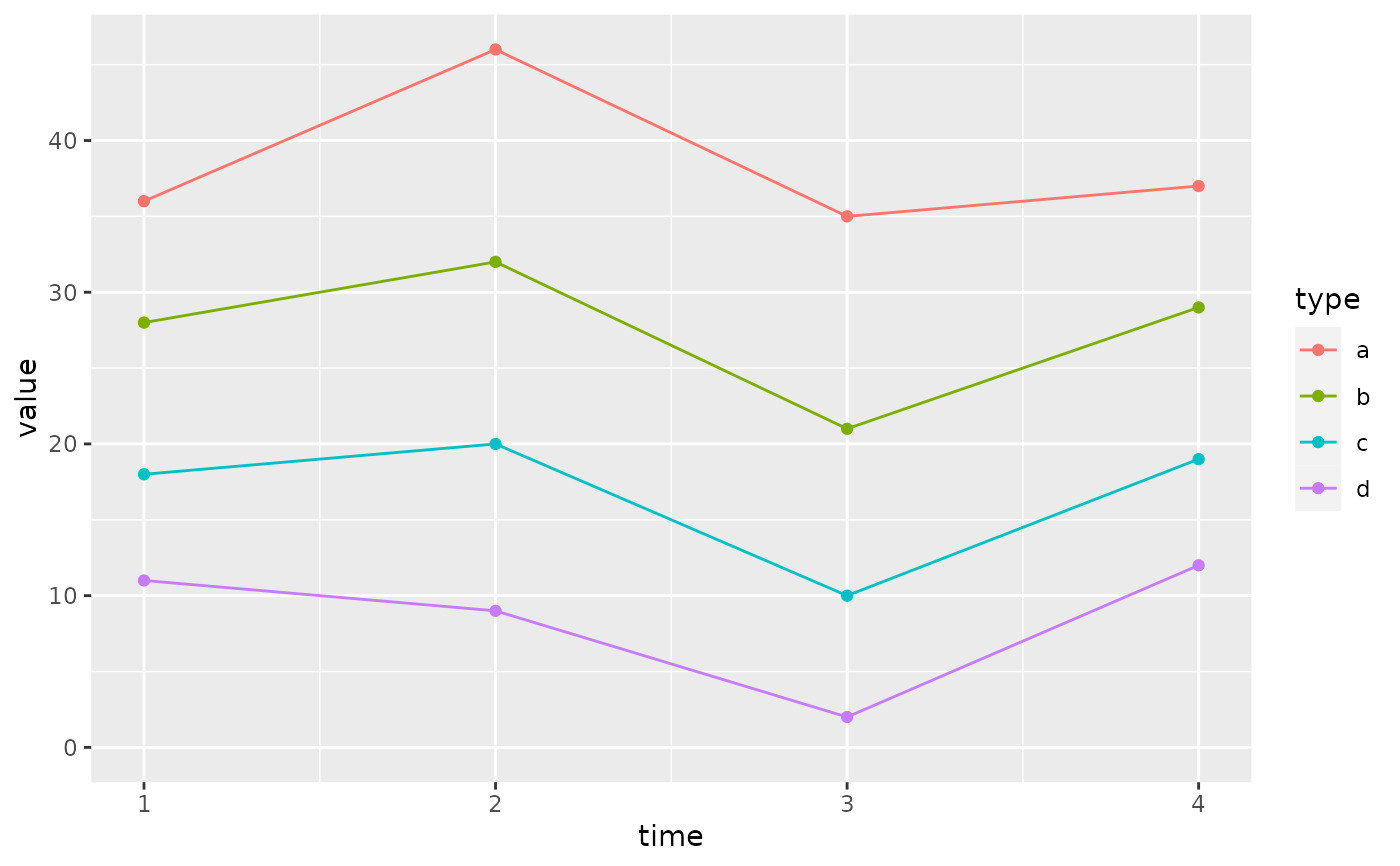
 # Non-area plots ------------------------------------------------------------
# When stacking across multiple layers it's a good idea to always set
# the `group` aesthetic in the ggplot() call. This ensures that all layers
# are stacked in the same way.
ggplot(series, aes(time, value, group = type)) +
geom_line(aes(colour = type), position = "stack") +
geom_point(aes(colour = type), position = "stack")
# Non-area plots ------------------------------------------------------------
# When stacking across multiple layers it's a good idea to always set
# the `group` aesthetic in the ggplot() call. This ensures that all layers
# are stacked in the same way.
ggplot(series, aes(time, value, group = type)) +
geom_line(aes(colour = type), position = "stack") +
geom_point(aes(colour = type), position = "stack")
 ggplot(series, aes(time, value, group = type)) +
geom_area(aes(fill = type)) +
geom_line(aes(group = type), position = "stack")
ggplot(series, aes(time, value, group = type)) +
geom_area(aes(fill = type)) +
geom_line(aes(group = type), position = "stack")
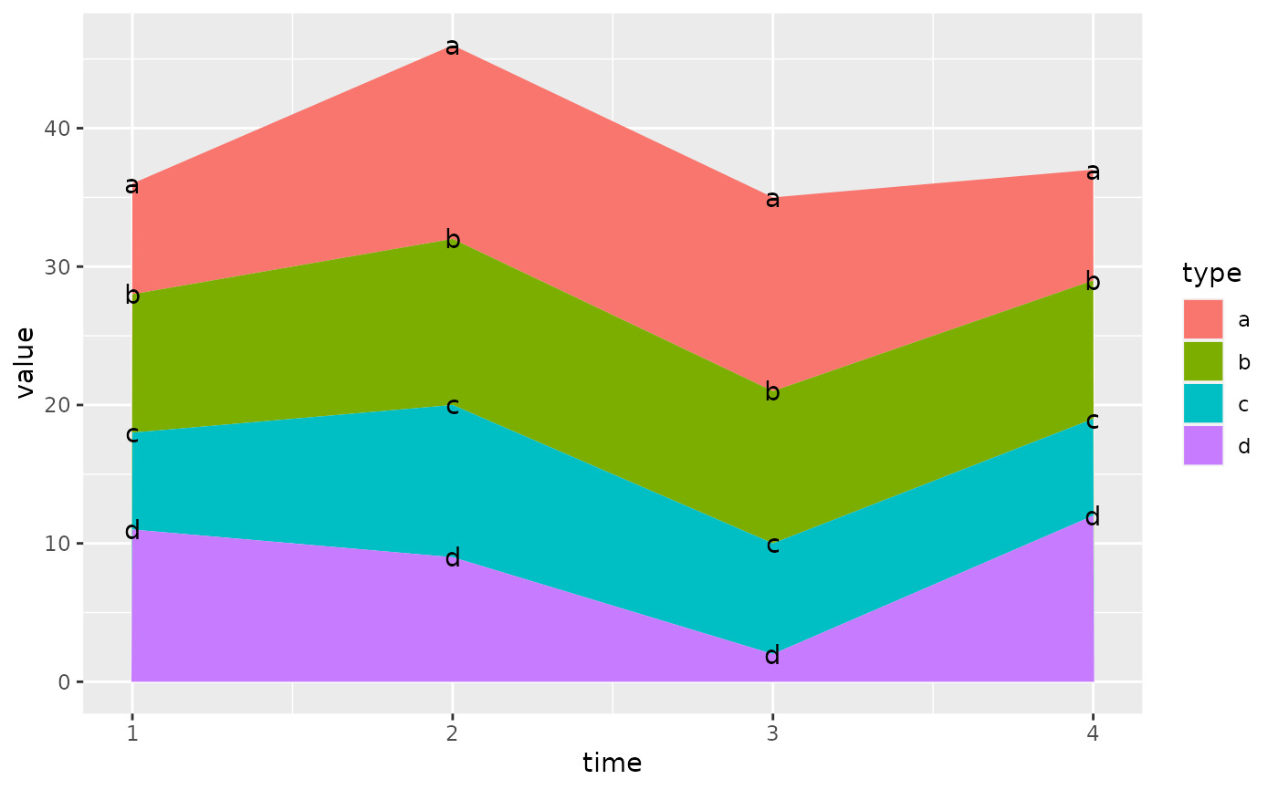
 # You can also stack labels, but the default position is suboptimal.
ggplot(series, aes(time, value, group = type)) +
geom_area(aes(fill = type)) +
geom_text(aes(label = type), position = "stack")
# You can also stack labels, but the default position is suboptimal.
ggplot(series, aes(time, value, group = type)) +
geom_area(aes(fill = type)) +
geom_text(aes(label = type), position = "stack")
 # You can override this with the vjust parameter. A vjust of 0.5
# will center the labels inside the corresponding area
ggplot(series, aes(time, value, group = type)) +
geom_area(aes(fill = type)) +
geom_text(aes(label = type), position = position_stack(vjust = 0.5))
# You can override this with the vjust parameter. A vjust of 0.5
# will center the labels inside the corresponding area
ggplot(series, aes(time, value, group = type)) +
geom_area(aes(fill = type)) +
geom_text(aes(label = type), position = position_stack(vjust = 0.5))
 # Negative values -----------------------------------------------------------
df <- tibble::tribble(
~x, ~y, ~grp,
"a", 1, "x",
"a", 2, "y",
"b", 1, "x",
"b", 3, "y",
"b", -1, "y"
)
ggplot(data = df, aes(x, y, group = grp)) +
geom_col(aes(fill = grp), position = position_stack(reverse = TRUE)) +
geom_hline(yintercept = 0)
# Negative values -----------------------------------------------------------
df <- tibble::tribble(
~x, ~y, ~grp,
"a", 1, "x",
"a", 2, "y",
"b", 1, "x",
"b", 3, "y",
"b", -1, "y"
)
ggplot(data = df, aes(x, y, group = grp)) +
geom_col(aes(fill = grp), position = position_stack(reverse = TRUE)) +
geom_hline(yintercept = 0)
 ggplot(data = df, aes(x, y, group = grp)) +
geom_col(aes(fill = grp)) +
geom_hline(yintercept = 0) +
geom_text(aes(label = grp), position = position_stack(vjust = 0.5))
ggplot(data = df, aes(x, y, group = grp)) +
geom_col(aes(fill = grp)) +
geom_hline(yintercept = 0) +
geom_text(aes(label = grp), position = position_stack(vjust = 0.5))
相關用法
- R ggplot2 position_dodge 躲避左右重疊的物體
- R ggplot2 position_nudge 將點微移固定距離
- R ggplot2 position_jitter 抖動點以避免過度繪製
- R ggplot2 position_jitterdodge 同時閃避和抖動
- R ggplot2 print.ggplot 明確繪製情節
- R ggplot2 print.ggproto 格式化或打印 ggproto 對象
- R ggplot2 annotation_logticks 注釋:記錄刻度線
- R ggplot2 vars 引用分麵變量
- R ggplot2 geom_qq 分位數-分位數圖
- R ggplot2 geom_spoke 由位置、方向和距離參數化的線段
- R ggplot2 geom_quantile 分位數回歸
- R ggplot2 geom_text 文本
- R ggplot2 get_alt_text 從繪圖中提取替代文本
- R ggplot2 annotation_custom 注釋:自定義grob
- R ggplot2 geom_ribbon 函數區和麵積圖
- R ggplot2 stat_ellipse 計算法行數據橢圓
- R ggplot2 resolution 計算數值向量的“分辨率”
- R ggplot2 geom_boxplot 盒須圖(Tukey 風格)
- R ggplot2 lims 設置規模限製
- R ggplot2 geom_hex 二維箱計數的六邊形熱圖
- R ggplot2 scale_gradient 漸變色階
- R ggplot2 scale_shape 形狀比例,又稱字形
- R ggplot2 geom_bar 條形圖
- R ggplot2 draw_key 圖例的關鍵字形
- R ggplot2 annotate 創建注釋層
注:本文由純淨天空篩選整理自Hadley Wickham等大神的英文原創作品 Stack overlapping objects on top of each another。非經特殊聲明,原始代碼版權歸原作者所有,本譯文未經允許或授權,請勿轉載或複製。