![[Superseded]](https://vimsky.com/wp-content/uploads/2023/09/4b45025dd0b01571ef2823327707b72d.svg)
coord_map() 使用 mapproj 包定義的任何投影將地球的一部分(近似球形)投影到平坦的 2D 平麵上。一般來說,Map投影不會保留直線,因此這需要大量的計算。 coord_quickmap() 是一種快速近似,可以保留直線。它最適合靠近赤道的較小區域。
coord_map() 和 coord_quickmap() 均被 coord_sf() 取代,並且不應再在新代碼中使用。通過 default_crs 參數設置默認坐標係,所有常規(非 sf)幾何圖形都可以與 coord_sf() 一起使用。另請參閱 annotation_map() 和 geom_map() 的示例。
用法
coord_map(
  projection = "mercator",
  ...,
  parameters = NULL,
  orientation = NULL,
  xlim = NULL,
  ylim = NULL,
  clip = "on"
)

coord_quickmap(xlim = NULL, ylim = NULL, expand = TRUE, clip = "on")
參數
- projection
-
要使用的投影,請參閱
mapproj::mapproject()列表 - ..., parameters
-
其他參數傳遞給
mapproj::mapproject()。使用...作為投影的命名參數,使用parameters作為未命名參數。如果存在parameters參數,則忽略...。 - orientation
-
投影方向,默認為
c(90, 0, mean(range(x)))。這對於許多投影來說並不是最佳的,因此您必須提供自己的投影。有關詳細信息,請參閱mapproj::mapproject()。 - xlim, ylim
-
手動指定 x/y 限製(以經度/緯度為單位)
- clip
-
是否應該將繪圖裁剪到繪圖麵板的範圍內?設置
"on"(默認)表示是,設置"off"表示否。詳情請參見coord_cartesian()。 - expand
-
如果
TRUE(默認值)會在限製中添加一個小的擴展因子,以確保數據和軸不重疊。如果FALSE,則完全從數據或xlim/ylim中獲取限製。
細節
Map投影必須考慮到赤道和極點之間經度的實際長度(以公裏為單位)不同這一事實。在赤道附近,1 度緯度與 1 度經度的長度之比約為 1。在極地附近,由於 1 度經度的長度趨於 0,因此趨於無窮大。對於跨度隻有幾米的地區,度並且不太靠近極點,將繪圖的縱橫比設置為適當的緯度/經度比近似於通常的墨卡托投影。這就是 coord_quickmap() 所做的,並且速度更快(特別是對於像 geom_tile() 這樣的複雜繪圖),但代價是正確性。
例子
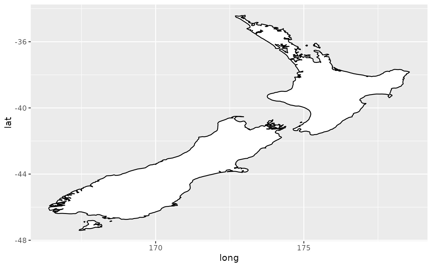
if (require("maps")) {
nz <- map_data("nz")
# Prepare a map of NZ
nzmap <- ggplot(nz, aes(x = long, y = lat, group = group)) +
geom_polygon(fill = "white", colour = "black")
# Plot it in cartesian coordinates
nzmap
}
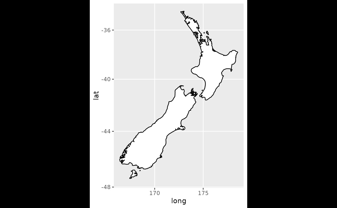
 if (require("maps")) {
# With correct mercator projection
nzmap + coord_map()
}
if (require("maps")) {
# With correct mercator projection
nzmap + coord_map()
}
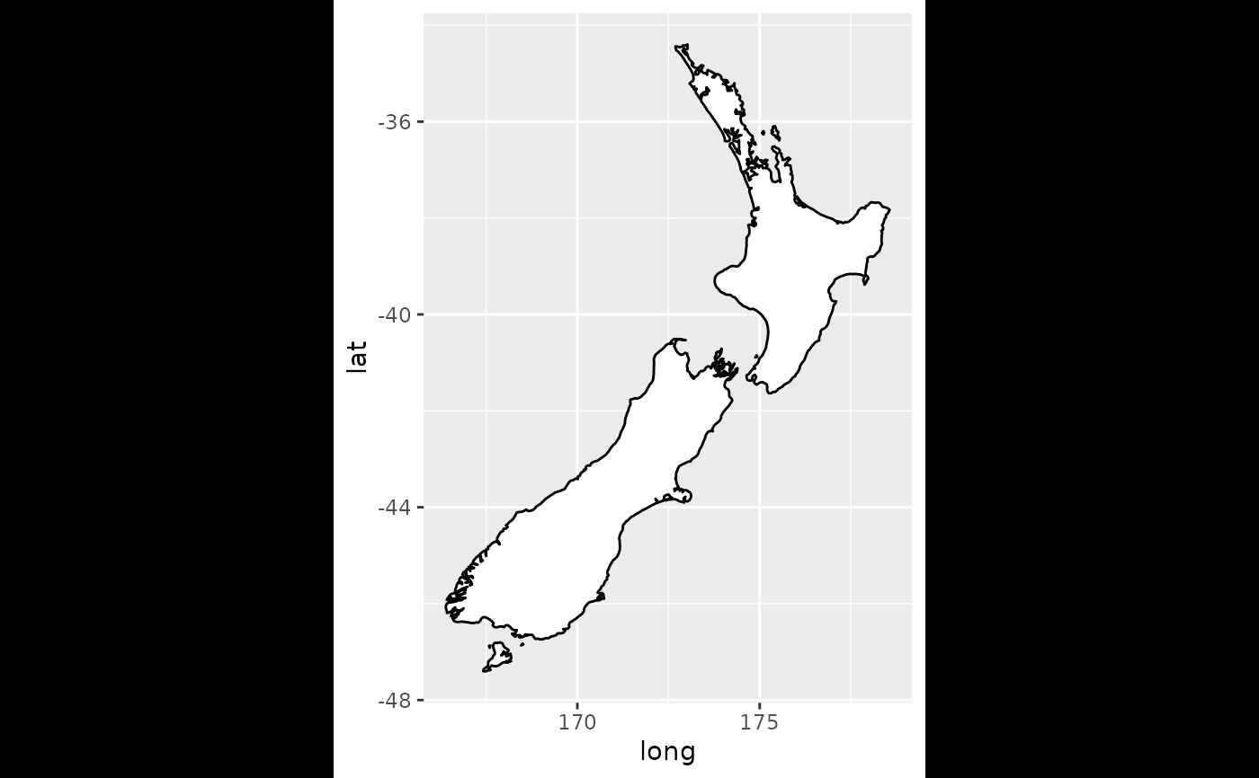
 if (require("maps")) {
# With the aspect ratio approximation
nzmap + coord_quickmap()
}
if (require("maps")) {
# With the aspect ratio approximation
nzmap + coord_quickmap()
}
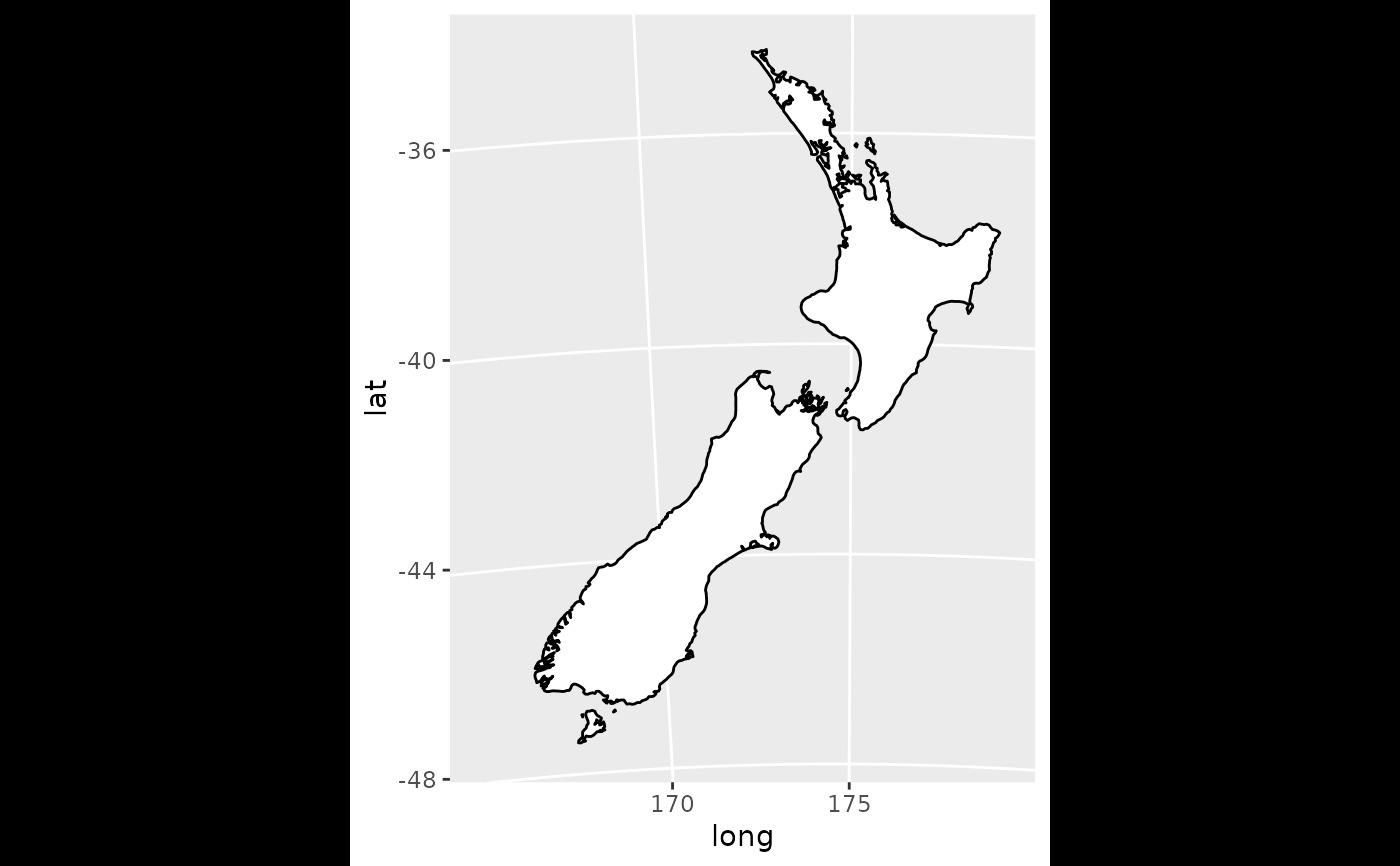
 if (require("maps")) {
# Other projections
nzmap + coord_map("azequalarea", orientation = c(-36.92, 174.6, 0))
}
if (require("maps")) {
# Other projections
nzmap + coord_map("azequalarea", orientation = c(-36.92, 174.6, 0))
}
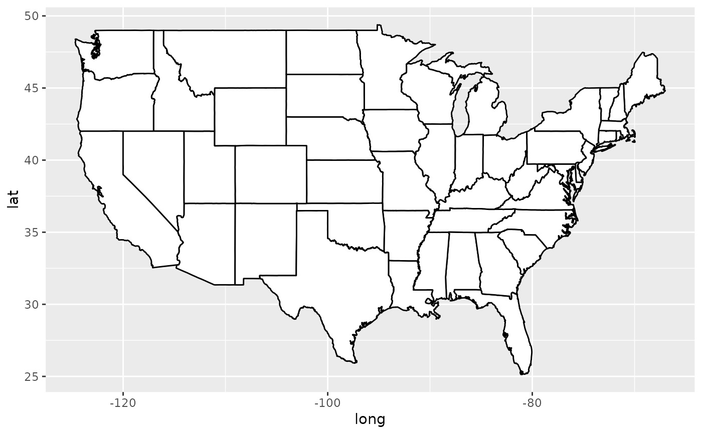
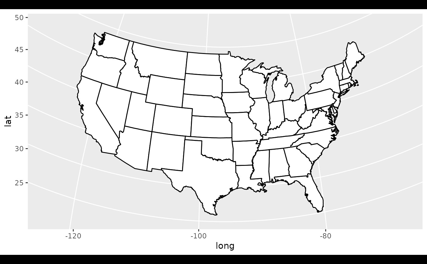
 if (require("maps")) {
states <- map_data("state")
usamap <- ggplot(states, aes(long, lat, group = group)) +
geom_polygon(fill = "white", colour = "black")
# Use cartesian coordinates
usamap
}
if (require("maps")) {
states <- map_data("state")
usamap <- ggplot(states, aes(long, lat, group = group)) +
geom_polygon(fill = "white", colour = "black")
# Use cartesian coordinates
usamap
}
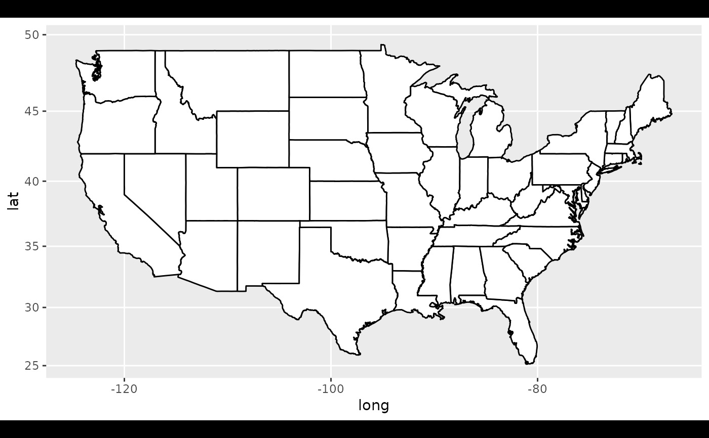
 if (require("maps")) {
# With mercator projection
usamap + coord_map()
}
if (require("maps")) {
# With mercator projection
usamap + coord_map()
}
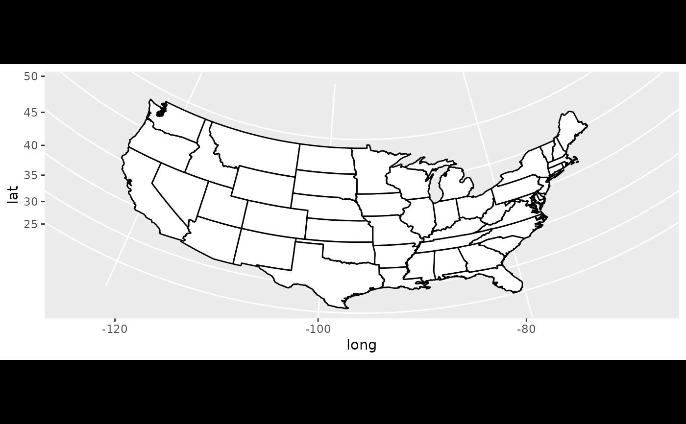
 if (require("maps")) {
# See ?mapproject for coordinate systems and their parameters
usamap + coord_map("gilbert")
}
if (require("maps")) {
# See ?mapproject for coordinate systems and their parameters
usamap + coord_map("gilbert")
}
 if (require("maps")) {
# For most projections, you'll need to set the orientation yourself
# as the automatic selection done by mapproject is not available to
# ggplot
usamap + coord_map("orthographic")
}
if (require("maps")) {
# For most projections, you'll need to set the orientation yourself
# as the automatic selection done by mapproject is not available to
# ggplot
usamap + coord_map("orthographic")
}
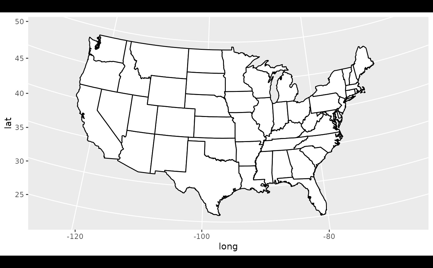
 if (require("maps")) {
usamap + coord_map("conic", lat0 = 30)
}
if (require("maps")) {
usamap + coord_map("conic", lat0 = 30)
}
 if (require("maps")) {
usamap + coord_map("bonne", lat0 = 50)
}
if (require("maps")) {
usamap + coord_map("bonne", lat0 = 50)
}
 if (FALSE) {
if (require("maps")) {
# World map, using geom_path instead of geom_polygon
world <- map_data("world")
worldmap <- ggplot(world, aes(x = long, y = lat, group = group)) +
geom_path() +
scale_y_continuous(breaks = (-2:2) * 30) +
scale_x_continuous(breaks = (-4:4) * 45)
# Orthographic projection with default orientation (looking down at North pole)
worldmap + coord_map("ortho")
}
if (require("maps")) {
# Looking up up at South Pole
worldmap + coord_map("ortho", orientation = c(-90, 0, 0))
}
if (require("maps")) {
# Centered on New York (currently has issues with closing polygons)
worldmap + coord_map("ortho", orientation = c(41, -74, 0))
}
}
if (FALSE) {
if (require("maps")) {
# World map, using geom_path instead of geom_polygon
world <- map_data("world")
worldmap <- ggplot(world, aes(x = long, y = lat, group = group)) +
geom_path() +
scale_y_continuous(breaks = (-2:2) * 30) +
scale_x_continuous(breaks = (-4:4) * 45)
# Orthographic projection with default orientation (looking down at North pole)
worldmap + coord_map("ortho")
}
if (require("maps")) {
# Looking up up at South Pole
worldmap + coord_map("ortho", orientation = c(-90, 0, 0))
}
if (require("maps")) {
# Centered on New York (currently has issues with closing polygons)
worldmap + coord_map("ortho", orientation = c(41, -74, 0))
}
}
相關用法
- R ggplot2 coord_fixed 具有固定“縱橫比”的笛卡爾坐標
- R ggplot2 coord_polar 極坐標
- R ggplot2 coord_cartesian 笛卡爾坐標
- R ggplot2 coord_trans 變換後的笛卡爾坐標係
- R ggplot2 coord_flip x 和 y 翻轉的笛卡爾坐標
- R ggplot2 cut_interval 將數值數據離散化為分類數據
- R ggplot2 annotation_logticks 注釋:記錄刻度線
- R ggplot2 vars 引用分麵變量
- R ggplot2 position_stack 將重疊的對象堆疊在一起
- R ggplot2 geom_qq 分位數-分位數圖
- R ggplot2 geom_spoke 由位置、方向和距離參數化的線段
- R ggplot2 geom_quantile 分位數回歸
- R ggplot2 geom_text 文本
- R ggplot2 get_alt_text 從繪圖中提取替代文本
- R ggplot2 annotation_custom 注釋:自定義grob
- R ggplot2 geom_ribbon 函數區和麵積圖
- R ggplot2 stat_ellipse 計算法行數據橢圓
- R ggplot2 resolution 計算數值向量的“分辨率”
- R ggplot2 geom_boxplot 盒須圖(Tukey 風格)
- R ggplot2 lims 設置規模限製
- R ggplot2 geom_hex 二維箱計數的六邊形熱圖
- R ggplot2 scale_gradient 漸變色階
- R ggplot2 scale_shape 形狀比例,又稱字形
- R ggplot2 geom_bar 條形圖
- R ggplot2 draw_key 圖例的關鍵字形
注:本文由純淨天空篩選整理自Hadley Wickham等大神的英文原創作品 Map projections。非經特殊聲明,原始代碼版權歸原作者所有,本譯文未經允許或授權,請勿轉載或複製。