本文簡要介紹 python 語言中 scipy.special.y1p_zeros 的用法。
用法:
scipy.special.y1p_zeros(nt, complex=False)#計算貝塞爾導數 Y1’(z) 的 nt 個零點,以及每個零點處的值。
這些值由每個 z1 處的 Y1(z1) 給出,其中 Y1’(z1)=0。
- nt: int
要返回的零數
- complex: 布爾值,默認為 False
設置為 False 僅返回實數零;設置為 True 僅返回具有負實部和正虛部的複數零。請注意,後者的複共軛也是函數的零,但此例程不返回。
- z1pn: ndarray
Y1'(z)的第n個零的位置
- y1z1pn: ndarray
第 n 個零的導數 Y1(z1) 值
參數 ::
返回 ::
參考:
[1]張善傑和金建明。 “特殊函數的計算”,John Wiley and Sons,1996 年,第 5 章。https://people.sc.fsu.edu/~jburkardt/f77_src/special_functions/special_functions.html
例子:
計算 的前四個根以及這些根處的 的值。
>>> import numpy as np >>> from scipy.special import y1p_zeros >>> y1grad_roots, y1_values = y1p_zeros(4) >>> with np.printoptions(precision=5): ... print(f"Y1' Roots: {y1grad_roots}") ... print(f"Y1 values: {y1_values}") Y1' Roots: [ 3.68302+0.j 6.9415 +0.j 10.1234 +0.j 13.28576+0.j] Y1 values: [ 0.41673+0.j -0.30317+0.j 0.25091+0.j -0.21897+0.j]y1p_zeros可以直接計算的極值點。在這裏,我們繪製 和前四個極值。>>> import matplotlib.pyplot as plt >>> from scipy.special import y1, yvp >>> y1_roots, y1_values_at_roots = y1p_zeros(4) >>> real_roots = y1_roots.real >>> xmax = 15 >>> x = np.linspace(0, xmax, 500) >>> x[0] += 1e-15 >>> fig, ax = plt.subplots() >>> ax.plot(x, y1(x), label=r'$Y_1$') >>> ax.plot(x, yvp(1, x, 1), label=r"$Y_1'$") >>> ax.scatter(real_roots, np.zeros((4, )), s=30, c='r', ... label=r"Roots of $Y_1'$", zorder=5) >>> ax.scatter(real_roots, y1_values_at_roots.real, s=30, c='k', ... label=r"Extrema of $Y_1$", zorder=5) >>> ax.hlines(0, 0, xmax, color='k') >>> ax.set_ylim(-0.5, 0.5) >>> ax.set_xlim(0, xmax) >>> ax.legend(ncol=2, bbox_to_anchor=(1., 0.75)) >>> plt.tight_layout() >>> plt.show()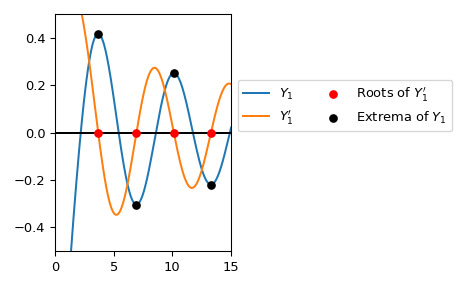
相關用法
- Python SciPy special.y1用法及代碼示例
- Python SciPy special.y1_zeros用法及代碼示例
- Python SciPy special.y0用法及代碼示例
- Python SciPy special.ynp_zeros用法及代碼示例
- Python SciPy special.yve用法及代碼示例
- Python SciPy special.yvp用法及代碼示例
- Python SciPy special.y0_zeros用法及代碼示例
- Python SciPy special.yn用法及代碼示例
- Python SciPy special.yv用法及代碼示例
- Python SciPy special.yn_zeros用法及代碼示例
- Python SciPy special.exp1用法及代碼示例
- Python SciPy special.expn用法及代碼示例
- Python SciPy special.ncfdtri用法及代碼示例
- Python SciPy special.gamma用法及代碼示例
- Python SciPy special.ellip_harm_2用法及代碼示例
- Python SciPy special.i1e用法及代碼示例
- Python SciPy special.smirnovi用法及代碼示例
- Python SciPy special.ker用法及代碼示例
- Python SciPy special.k0e用法及代碼示例
- Python SciPy special.j1用法及代碼示例
- Python SciPy special.logsumexp用法及代碼示例
- Python SciPy special.expit用法及代碼示例
- Python SciPy special.polygamma用法及代碼示例
- Python SciPy special.nbdtrik用法及代碼示例
- Python SciPy special.nbdtrin用法及代碼示例
注:本文由純淨天空篩選整理自scipy.org大神的英文原創作品 scipy.special.y1p_zeros。非經特殊聲明,原始代碼版權歸原作者所有,本譯文未經允許或授權,請勿轉載或複製。