Augment 接受模型对象和数据集,并添加有关数据集中每个观察值的信息。最常见的是,这包括 .fitted 列中的预测值、.resid 列中的残差以及 .se.fit 列中拟合值的标准误差。新列始终以 . 前缀开头,以避免覆盖原始数据集中的列。
用户可以通过 data 参数或 newdata 参数传递数据以进行增强。如果用户将数据传递给 data 参数,则它必须正是用于拟合模型对象的数据。将数据集传递给 newdata 以扩充模型拟合期间未使用的数据。这仍然要求至少存在用于拟合模型的所有预测变量列。如果用于拟合模型的原始结果变量未包含在 newdata 中,则输出中不会包含 .resid 列。
根据是否给出 data 或 newdata,增强的行为通常会有所不同。这是因为通常存在与训练观察(例如影响或相关)测量相关的信息,而这些信息对于新观察没有有意义的定义。
为了方便起见,许多增强方法提供默认的 data 参数,以便 augment(fit) 将返回增强的训练数据。在这些情况下,augment 尝试根据模型对象重建原始数据,并取得了不同程度的成功。
增强数据集始终以 tibble::tibble 形式返回,其行数与传递的数据集相同。这意味着传递的数据必须可强制转换为 tibble。如果预测变量将模型作为协变量矩阵的一部分输入,例如当模型公式使用 splines::ns() 、 stats::poly() 或 survival::Surv() 时,它会表示为矩阵列。
我们正在定义适合各种 na.action 参数的模型的行为,但目前不保证数据丢失时的行为。
用法
# S3 method for lm
augment(
  x,
  data = model.frame(x),
  newdata = NULL,
  se_fit = FALSE,
  interval = c("none", "confidence", "prediction"),
  ...
)
参数
- x
-
由
stats::lm()创建的lm对象。 - data
-
base::data.frame 或
tibble::tibble()包含用于生成对象x的原始数据。默认为stats::model.frame(x),以便augment(my_fit)返回增强的原始数据。不要将新数据传递给data参数。增强将报告传递给data参数的数据的影响和烹饪距离等信息。这些度量仅针对原始训练数据定义。 - newdata
-
base::data.frame()或tibble::tibble()包含用于创建x的所有原始预测变量。默认为NULL,表示没有任何内容传递给newdata。如果指定了newdata,则data参数将被忽略。 - se_fit
-
逻辑指示是否应将
.se.fit列添加到增强输出中。对于某些模型,此计算可能有点耗时。默认为FALSE。 - interval
-
指示要添加到增强输出的置信区间列类型的字符。传递给
predict(),默认为"none"。 - ...
-
附加参数。不曾用过。仅需要匹配通用签名。注意:拼写错误的参数将被吸收到
...中,并被忽略。如果拼写错误的参数有默认值,则将使用默认值。例如,如果您传递conf.lvel = 0.9,所有计算将使用conf.level = 0.95进行。这里有两个异常:
细节
当使用 na.action = "na.omit" 执行建模时(这是典型的默认设置),初始数据中带有 NA 的行将完全从增强 DataFrame 中省略。当使用 na.action = "na.exclude" 执行建模时,应提供原始数据作为第二个参数,此时增强数据将包含这些行(通常用 NA 代替新列)。如果未向 augment() 和 na.action = "na.exclude" 提供原始数据,则会引发警告并删除不完整的行。
一些不寻常的 lm 对象(例如 MASS 中的 rlm)可能会省略 .cooksd 和 .std.resid 。 mgcv 中的 gam 省略 .sigma 。
当提供 newdata 时,仅返回 .fitted 、 .resid 和 .se.fit 列。
也可以看看
augment() , stats::predict.lm()
其他电影整理者:augment.glm() , glance.glm() , glance.lm() , glance.summary.lm() , glance.svyglm() , tidy.glm() , tidy.lm.beta() , tidy.lm() , tidy.mlm() , tidy.summary.lm()
值
带有列的 tibble::tibble():
- .cooksd
-
厨师距离。
- .fitted
-
拟合值或预测值。
- .hat
-
帽子矩阵的对角线。
- .lower
-
拟合值的区间下限。
- .resid
-
观察值和拟合值之间的差异。
- .se.fit
-
拟合值的标准误差。
- .sigma
-
从模型中删除相应观测值时的估计残差标准差。
- .std.resid
-
标准化残差。
- .upper
-
拟合值的区间上限。
例子
library(ggplot2)
library(dplyr)
mod <- lm(mpg ~ wt + qsec, data = mtcars)
tidy(mod)
#> # A tibble: 3 × 5
#> term estimate std.error statistic p.value
#> <chr> <dbl> <dbl> <dbl> <dbl>
#> 1 (Intercept) 19.7 5.25 3.76 7.65e- 4
#> 2 wt -5.05 0.484 -10.4 2.52e-11
#> 3 qsec 0.929 0.265 3.51 1.50e- 3
glance(mod)
#> # A tibble: 1 × 12
#> r.squared adj.r.squared sigma statistic p.value df logLik AIC
#> <dbl> <dbl> <dbl> <dbl> <dbl> <dbl> <dbl> <dbl>
#> 1 0.826 0.814 2.60 69.0 9.39e-12 2 -74.4 157.
#> # ℹ 4 more variables: BIC <dbl>, deviance <dbl>, df.residual <int>,
#> # nobs <int>
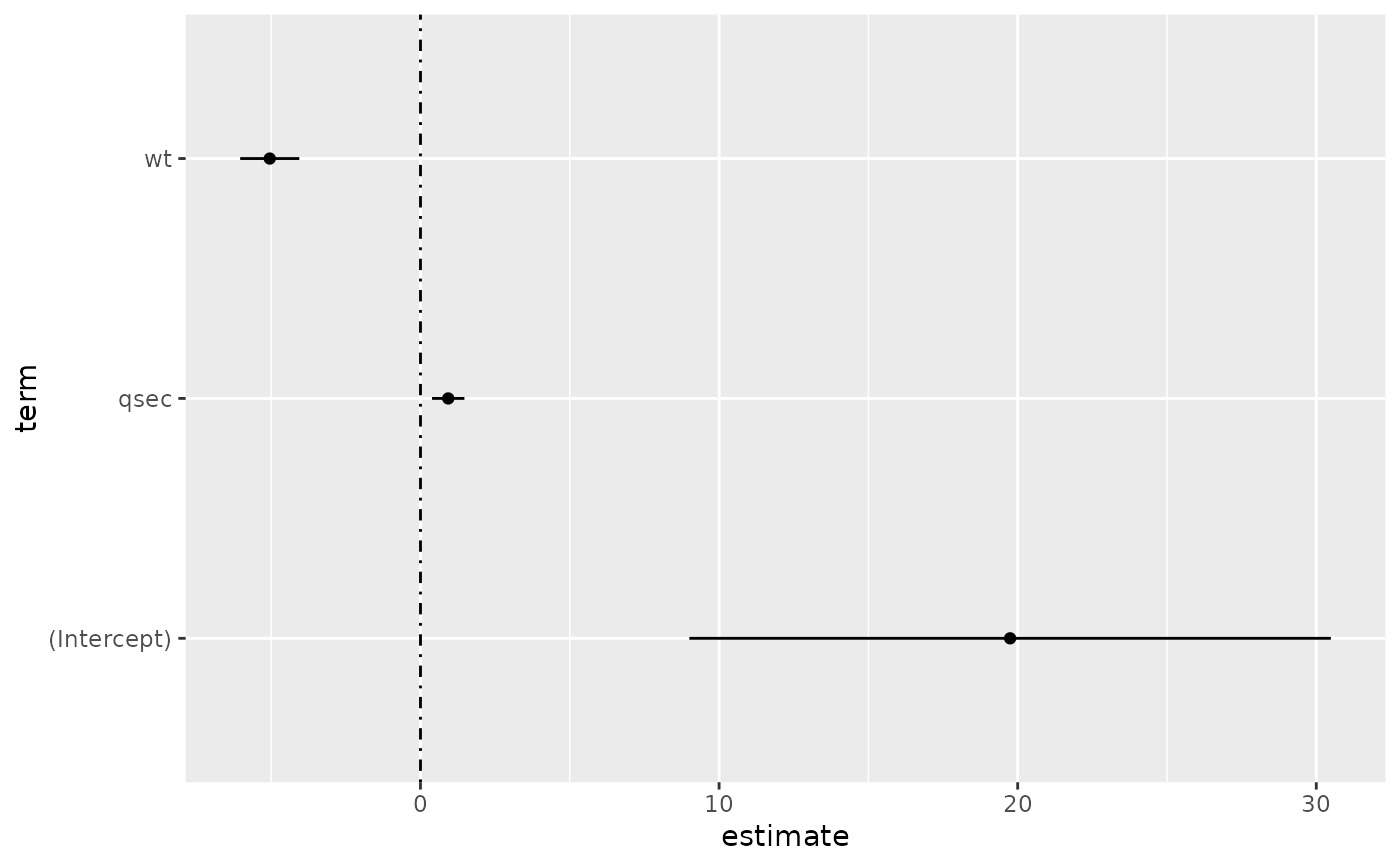
# coefficient plot
d <- tidy(mod, conf.int = TRUE)
ggplot(d, aes(estimate, term, xmin = conf.low, xmax = conf.high, height = 0)) +
geom_point() +
geom_vline(xintercept = 0, lty = 4) +
geom_errorbarh()
 # aside: There are tidy() and glance() methods for lm.summary objects too.
# this can be useful when you want to conserve memory by converting large lm
# objects into their leaner summary.lm equivalents.
s <- summary(mod)
tidy(s, conf.int = TRUE)
#> # A tibble: 3 × 7
#> term estimate std.error statistic p.value conf.low conf.high
#> <chr> <dbl> <dbl> <dbl> <dbl> <dbl> <dbl>
#> 1 (Intercept) 19.7 5.25 3.76 7.65e- 4 9.00 30.5
#> 2 wt -5.05 0.484 -10.4 2.52e-11 -6.04 -4.06
#> 3 qsec 0.929 0.265 3.51 1.50e- 3 0.387 1.47
glance(s)
#> # A tibble: 1 × 8
#> r.squared adj.r.squared sigma statistic p.value df df.residual nobs
#> <dbl> <dbl> <dbl> <dbl> <dbl> <dbl> <int> <dbl>
#> 1 0.826 0.814 2.60 69.0 9.39e-12 2 29 32
augment(mod)
#> # A tibble: 32 × 10
#> .rownames mpg wt qsec .fitted .resid .hat .sigma .cooksd
#> <chr> <dbl> <dbl> <dbl> <dbl> <dbl> <dbl> <dbl> <dbl>
#> 1 Mazda RX4 21 2.62 16.5 21.8 -0.815 0.0693 2.64 2.63e-3
#> 2 Mazda RX4 Wag 21 2.88 17.0 21.0 -0.0482 0.0444 2.64 5.59e-6
#> 3 Datsun 710 22.8 2.32 18.6 25.3 -2.53 0.0607 2.60 2.17e-2
#> 4 Hornet 4 Drive 21.4 3.22 19.4 21.6 -0.181 0.0576 2.64 1.05e-4
#> 5 Hornet Sportab… 18.7 3.44 17.0 18.2 0.504 0.0389 2.64 5.29e-4
#> 6 Valiant 18.1 3.46 20.2 21.1 -2.97 0.0957 2.58 5.10e-2
#> 7 Duster 360 14.3 3.57 15.8 16.4 -2.14 0.0729 2.61 1.93e-2
#> 8 Merc 240D 24.4 3.19 20 22.2 2.17 0.0791 2.61 2.18e-2
#> 9 Merc 230 22.8 3.15 22.9 25.1 -2.32 0.295 2.59 1.59e-1
#> 10 Merc 280 19.2 3.44 18.3 19.4 -0.185 0.0358 2.64 6.55e-5
#> # ℹ 22 more rows
#> # ℹ 1 more variable: .std.resid <dbl>
augment(mod, mtcars, interval = "confidence")
#> # A tibble: 32 × 20
#> .rownames mpg cyl disp hp drat wt qsec vs am gear
#> <chr> <dbl> <dbl> <dbl> <dbl> <dbl> <dbl> <dbl> <dbl> <dbl> <dbl>
#> 1 Mazda RX4 21 6 160 110 3.9 2.62 16.5 0 1 4
#> 2 Mazda RX4 … 21 6 160 110 3.9 2.88 17.0 0 1 4
#> 3 Datsun 710 22.8 4 108 93 3.85 2.32 18.6 1 1 4
#> 4 Hornet 4 D… 21.4 6 258 110 3.08 3.22 19.4 1 0 3
#> 5 Hornet Spo… 18.7 8 360 175 3.15 3.44 17.0 0 0 3
#> 6 Valiant 18.1 6 225 105 2.76 3.46 20.2 1 0 3
#> 7 Duster 360 14.3 8 360 245 3.21 3.57 15.8 0 0 3
#> 8 Merc 240D 24.4 4 147. 62 3.69 3.19 20 1 0 4
#> 9 Merc 230 22.8 4 141. 95 3.92 3.15 22.9 1 0 4
#> 10 Merc 280 19.2 6 168. 123 3.92 3.44 18.3 1 0 4
#> # ℹ 22 more rows
#> # ℹ 9 more variables: carb <dbl>, .fitted <dbl>, .lower <dbl>,
#> # .upper <dbl>, .resid <dbl>, .hat <dbl>, .sigma <dbl>, .cooksd <dbl>,
#> # .std.resid <dbl>
# predict on new data
newdata <- mtcars %>%
head(6) %>%
mutate(wt = wt + 1)
augment(mod, newdata = newdata)
#> # A tibble: 6 × 14
#> .rownames mpg cyl disp hp drat wt qsec vs am gear
#> <chr> <dbl> <dbl> <dbl> <dbl> <dbl> <dbl> <dbl> <dbl> <dbl> <dbl>
#> 1 Mazda RX4 21 6 160 110 3.9 3.62 16.5 0 1 4
#> 2 Mazda RX4 W… 21 6 160 110 3.9 3.88 17.0 0 1 4
#> 3 Datsun 710 22.8 4 108 93 3.85 3.32 18.6 1 1 4
#> 4 Hornet 4 Dr… 21.4 6 258 110 3.08 4.22 19.4 1 0 3
#> 5 Hornet Spor… 18.7 8 360 175 3.15 4.44 17.0 0 0 3
#> 6 Valiant 18.1 6 225 105 2.76 4.46 20.2 1 0 3
#> # ℹ 3 more variables: carb <dbl>, .fitted <dbl>, .resid <dbl>
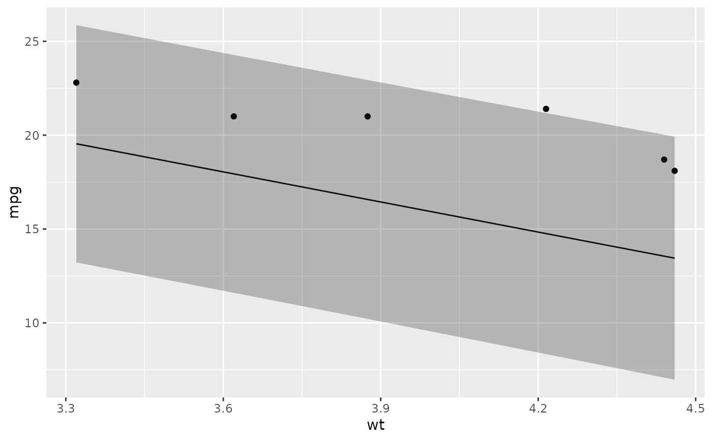
# ggplot2 example where we also construct 95% prediction interval
# simpler bivariate model since we're plotting in 2D
mod2 <- lm(mpg ~ wt, data = mtcars)
au <- augment(mod2, newdata = newdata, interval = "prediction")
ggplot(au, aes(wt, mpg)) +
geom_point() +
geom_line(aes(y = .fitted)) +
geom_ribbon(aes(ymin = .lower, ymax = .upper), col = NA, alpha = 0.3)
# aside: There are tidy() and glance() methods for lm.summary objects too.
# this can be useful when you want to conserve memory by converting large lm
# objects into their leaner summary.lm equivalents.
s <- summary(mod)
tidy(s, conf.int = TRUE)
#> # A tibble: 3 × 7
#> term estimate std.error statistic p.value conf.low conf.high
#> <chr> <dbl> <dbl> <dbl> <dbl> <dbl> <dbl>
#> 1 (Intercept) 19.7 5.25 3.76 7.65e- 4 9.00 30.5
#> 2 wt -5.05 0.484 -10.4 2.52e-11 -6.04 -4.06
#> 3 qsec 0.929 0.265 3.51 1.50e- 3 0.387 1.47
glance(s)
#> # A tibble: 1 × 8
#> r.squared adj.r.squared sigma statistic p.value df df.residual nobs
#> <dbl> <dbl> <dbl> <dbl> <dbl> <dbl> <int> <dbl>
#> 1 0.826 0.814 2.60 69.0 9.39e-12 2 29 32
augment(mod)
#> # A tibble: 32 × 10
#> .rownames mpg wt qsec .fitted .resid .hat .sigma .cooksd
#> <chr> <dbl> <dbl> <dbl> <dbl> <dbl> <dbl> <dbl> <dbl>
#> 1 Mazda RX4 21 2.62 16.5 21.8 -0.815 0.0693 2.64 2.63e-3
#> 2 Mazda RX4 Wag 21 2.88 17.0 21.0 -0.0482 0.0444 2.64 5.59e-6
#> 3 Datsun 710 22.8 2.32 18.6 25.3 -2.53 0.0607 2.60 2.17e-2
#> 4 Hornet 4 Drive 21.4 3.22 19.4 21.6 -0.181 0.0576 2.64 1.05e-4
#> 5 Hornet Sportab… 18.7 3.44 17.0 18.2 0.504 0.0389 2.64 5.29e-4
#> 6 Valiant 18.1 3.46 20.2 21.1 -2.97 0.0957 2.58 5.10e-2
#> 7 Duster 360 14.3 3.57 15.8 16.4 -2.14 0.0729 2.61 1.93e-2
#> 8 Merc 240D 24.4 3.19 20 22.2 2.17 0.0791 2.61 2.18e-2
#> 9 Merc 230 22.8 3.15 22.9 25.1 -2.32 0.295 2.59 1.59e-1
#> 10 Merc 280 19.2 3.44 18.3 19.4 -0.185 0.0358 2.64 6.55e-5
#> # ℹ 22 more rows
#> # ℹ 1 more variable: .std.resid <dbl>
augment(mod, mtcars, interval = "confidence")
#> # A tibble: 32 × 20
#> .rownames mpg cyl disp hp drat wt qsec vs am gear
#> <chr> <dbl> <dbl> <dbl> <dbl> <dbl> <dbl> <dbl> <dbl> <dbl> <dbl>
#> 1 Mazda RX4 21 6 160 110 3.9 2.62 16.5 0 1 4
#> 2 Mazda RX4 … 21 6 160 110 3.9 2.88 17.0 0 1 4
#> 3 Datsun 710 22.8 4 108 93 3.85 2.32 18.6 1 1 4
#> 4 Hornet 4 D… 21.4 6 258 110 3.08 3.22 19.4 1 0 3
#> 5 Hornet Spo… 18.7 8 360 175 3.15 3.44 17.0 0 0 3
#> 6 Valiant 18.1 6 225 105 2.76 3.46 20.2 1 0 3
#> 7 Duster 360 14.3 8 360 245 3.21 3.57 15.8 0 0 3
#> 8 Merc 240D 24.4 4 147. 62 3.69 3.19 20 1 0 4
#> 9 Merc 230 22.8 4 141. 95 3.92 3.15 22.9 1 0 4
#> 10 Merc 280 19.2 6 168. 123 3.92 3.44 18.3 1 0 4
#> # ℹ 22 more rows
#> # ℹ 9 more variables: carb <dbl>, .fitted <dbl>, .lower <dbl>,
#> # .upper <dbl>, .resid <dbl>, .hat <dbl>, .sigma <dbl>, .cooksd <dbl>,
#> # .std.resid <dbl>
# predict on new data
newdata <- mtcars %>%
head(6) %>%
mutate(wt = wt + 1)
augment(mod, newdata = newdata)
#> # A tibble: 6 × 14
#> .rownames mpg cyl disp hp drat wt qsec vs am gear
#> <chr> <dbl> <dbl> <dbl> <dbl> <dbl> <dbl> <dbl> <dbl> <dbl> <dbl>
#> 1 Mazda RX4 21 6 160 110 3.9 3.62 16.5 0 1 4
#> 2 Mazda RX4 W… 21 6 160 110 3.9 3.88 17.0 0 1 4
#> 3 Datsun 710 22.8 4 108 93 3.85 3.32 18.6 1 1 4
#> 4 Hornet 4 Dr… 21.4 6 258 110 3.08 4.22 19.4 1 0 3
#> 5 Hornet Spor… 18.7 8 360 175 3.15 4.44 17.0 0 0 3
#> 6 Valiant 18.1 6 225 105 2.76 4.46 20.2 1 0 3
#> # ℹ 3 more variables: carb <dbl>, .fitted <dbl>, .resid <dbl>
# ggplot2 example where we also construct 95% prediction interval
# simpler bivariate model since we're plotting in 2D
mod2 <- lm(mpg ~ wt, data = mtcars)
au <- augment(mod2, newdata = newdata, interval = "prediction")
ggplot(au, aes(wt, mpg)) +
geom_point() +
geom_line(aes(y = .fitted)) +
geom_ribbon(aes(ymin = .lower, ymax = .upper), col = NA, alpha = 0.3)
 # predict on new data without outcome variable. Output does not include .resid
newdata <- newdata %>%
select(-mpg)
#> Error in select(., -mpg): unused argument (-mpg)
augment(mod, newdata = newdata)
#> # A tibble: 6 × 14
#> .rownames mpg cyl disp hp drat wt qsec vs am gear
#> <chr> <dbl> <dbl> <dbl> <dbl> <dbl> <dbl> <dbl> <dbl> <dbl> <dbl>
#> 1 Mazda RX4 21 6 160 110 3.9 3.62 16.5 0 1 4
#> 2 Mazda RX4 W… 21 6 160 110 3.9 3.88 17.0 0 1 4
#> 3 Datsun 710 22.8 4 108 93 3.85 3.32 18.6 1 1 4
#> 4 Hornet 4 Dr… 21.4 6 258 110 3.08 4.22 19.4 1 0 3
#> 5 Hornet Spor… 18.7 8 360 175 3.15 4.44 17.0 0 0 3
#> 6 Valiant 18.1 6 225 105 2.76 4.46 20.2 1 0 3
#> # ℹ 3 more variables: carb <dbl>, .fitted <dbl>, .resid <dbl>
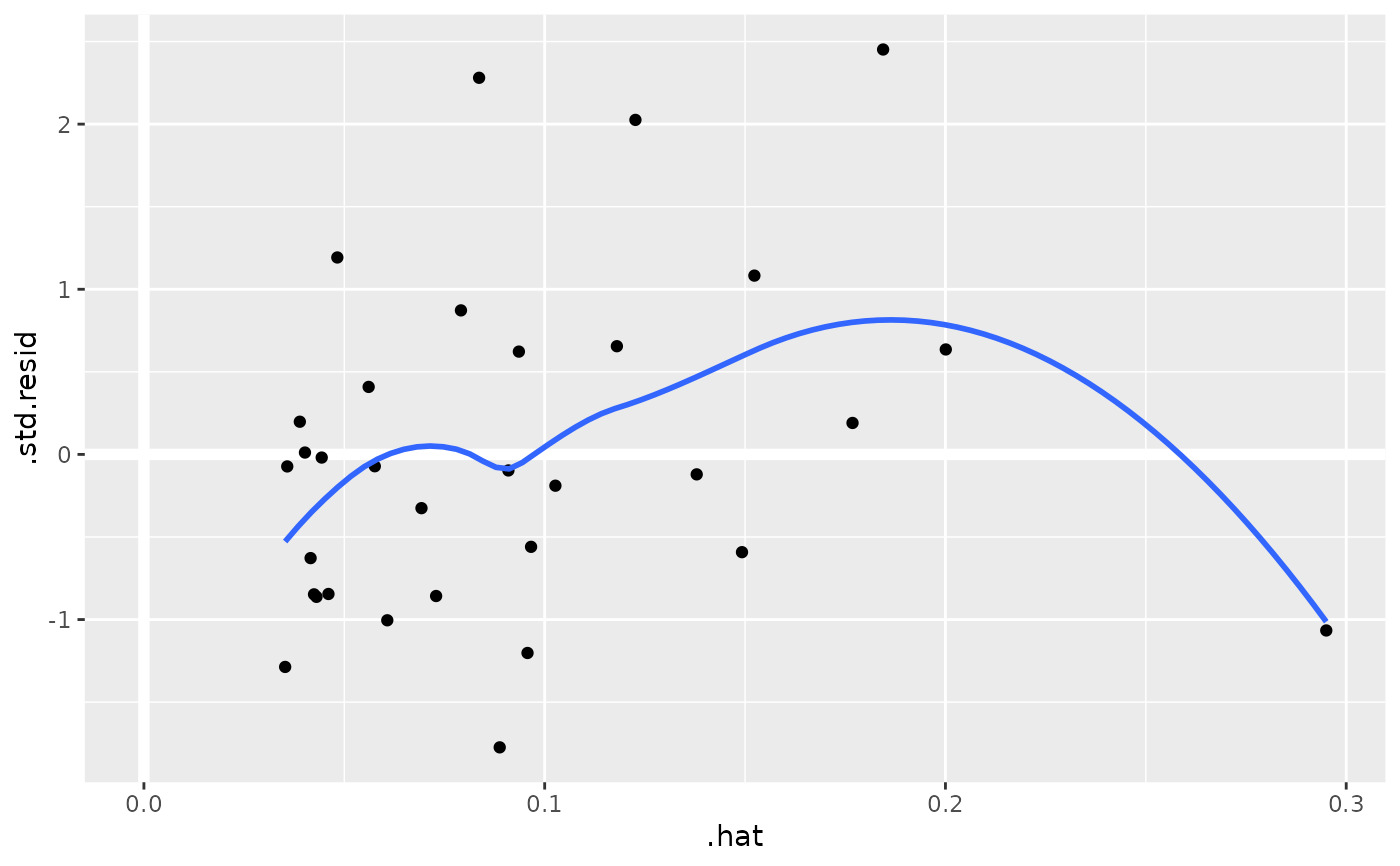
au <- augment(mod, data = mtcars)
ggplot(au, aes(.hat, .std.resid)) +
geom_vline(size = 2, colour = "white", xintercept = 0) +
geom_hline(size = 2, colour = "white", yintercept = 0) +
geom_point() +
geom_smooth(se = FALSE)
#> Warning: Using `size` aesthetic for lines was deprecated in ggplot2 3.4.0.
#> ℹ Please use `linewidth` instead.
#> `geom_smooth()` using method = 'loess' and formula = 'y ~ x'
# predict on new data without outcome variable. Output does not include .resid
newdata <- newdata %>%
select(-mpg)
#> Error in select(., -mpg): unused argument (-mpg)
augment(mod, newdata = newdata)
#> # A tibble: 6 × 14
#> .rownames mpg cyl disp hp drat wt qsec vs am gear
#> <chr> <dbl> <dbl> <dbl> <dbl> <dbl> <dbl> <dbl> <dbl> <dbl> <dbl>
#> 1 Mazda RX4 21 6 160 110 3.9 3.62 16.5 0 1 4
#> 2 Mazda RX4 W… 21 6 160 110 3.9 3.88 17.0 0 1 4
#> 3 Datsun 710 22.8 4 108 93 3.85 3.32 18.6 1 1 4
#> 4 Hornet 4 Dr… 21.4 6 258 110 3.08 4.22 19.4 1 0 3
#> 5 Hornet Spor… 18.7 8 360 175 3.15 4.44 17.0 0 0 3
#> 6 Valiant 18.1 6 225 105 2.76 4.46 20.2 1 0 3
#> # ℹ 3 more variables: carb <dbl>, .fitted <dbl>, .resid <dbl>
au <- augment(mod, data = mtcars)
ggplot(au, aes(.hat, .std.resid)) +
geom_vline(size = 2, colour = "white", xintercept = 0) +
geom_hline(size = 2, colour = "white", yintercept = 0) +
geom_point() +
geom_smooth(se = FALSE)
#> Warning: Using `size` aesthetic for lines was deprecated in ggplot2 3.4.0.
#> ℹ Please use `linewidth` instead.
#> `geom_smooth()` using method = 'loess' and formula = 'y ~ x'
 plot(mod, which = 6)
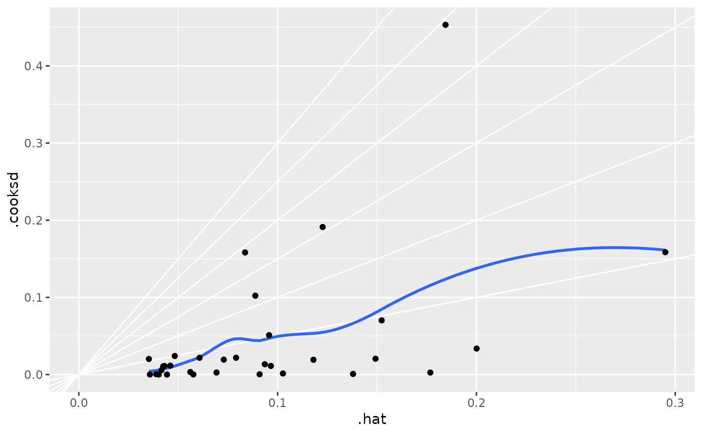
 ggplot(au, aes(.hat, .cooksd)) +
geom_vline(xintercept = 0, colour = NA) +
geom_abline(slope = seq(0, 3, by = 0.5), colour = "white") +
geom_smooth(se = FALSE) +
geom_point()
#> `geom_smooth()` using method = 'loess' and formula = 'y ~ x'
ggplot(au, aes(.hat, .cooksd)) +
geom_vline(xintercept = 0, colour = NA) +
geom_abline(slope = seq(0, 3, by = 0.5), colour = "white") +
geom_smooth(se = FALSE) +
geom_point()
#> `geom_smooth()` using method = 'loess' and formula = 'y ~ x'
 # column-wise models
a <- matrix(rnorm(20), nrow = 10)
b <- a + rnorm(length(a))
result <- lm(b ~ a)
tidy(result)
#> # A tibble: 6 × 6
#> response term estimate std.error statistic p.value
#> <chr> <chr> <dbl> <dbl> <dbl> <dbl>
#> 1 Y1 (Intercept) -0.292 0.280 -1.04 0.332
#> 2 Y1 a1 1.28 0.232 5.50 0.000903
#> 3 Y1 a2 -0.519 0.187 -2.78 0.0274
#> 4 Y2 (Intercept) -0.0923 0.259 -0.357 0.732
#> 5 Y2 a1 -0.231 0.214 -1.08 0.317
#> 6 Y2 a2 0.768 0.172 4.45 0.00296
# column-wise models
a <- matrix(rnorm(20), nrow = 10)
b <- a + rnorm(length(a))
result <- lm(b ~ a)
tidy(result)
#> # A tibble: 6 × 6
#> response term estimate std.error statistic p.value
#> <chr> <chr> <dbl> <dbl> <dbl> <dbl>
#> 1 Y1 (Intercept) -0.292 0.280 -1.04 0.332
#> 2 Y1 a1 1.28 0.232 5.50 0.000903
#> 3 Y1 a2 -0.519 0.187 -2.78 0.0274
#> 4 Y2 (Intercept) -0.0923 0.259 -0.357 0.732
#> 5 Y2 a1 -0.231 0.214 -1.08 0.317
#> 6 Y2 a2 0.768 0.172 4.45 0.00296
相关用法
- R broom augment.lmRob 使用来自 lmRob 对象的信息增强数据
- R broom augment.loess 整理 a(n) 黄土对象
- R broom augment.betamfx 使用来自 betamfx 对象的信息增强数据
- R broom augment.robustbase.glmrob 使用来自 glmrob 对象的信息增强数据
- R broom augment.rlm 使用来自 rlm 对象的信息增强数据
- R broom augment.htest 使用来自(n)个 htest 对象的信息来增强数据
- R broom augment.clm 使用来自 clm 对象的信息增强数据
- R broom augment.speedlm 使用来自 speedlm 对象的信息增强数据
- R broom augment.felm 使用来自 (n) 个 felm 对象的信息来增强数据
- R broom augment.smooth.spline 整理一个(n)smooth.spline对象
- R broom augment.drc 使用来自 a(n) drc 对象的信息增强数据
- R broom augment.decomposed.ts 使用来自 decomposed.ts 对象的信息增强数据
- R broom augment.poLCA 使用来自 poLCA 对象的信息增强数据
- R broom augment.rqs 使用来自 (n) 个 rqs 对象的信息来增强数据
- R broom augment.polr 使用来自 (n) 个 polr 对象的信息增强数据
- R broom augment.plm 使用来自 plm 对象的信息增强数据
- R broom augment.nls 使用来自 nls 对象的信息增强数据
- R broom augment.gam 使用来自 gam 对象的信息增强数据
- R broom augment.fixest 使用来自(n)个最固定对象的信息来增强数据
- R broom augment.survreg 使用来自 survreg 对象的信息增强数据
- R broom augment.rq 使用来自 a(n) rq 对象的信息增强数据
- R broom augment.Mclust 使用来自 Mclust 对象的信息增强数据
- R broom augment.nlrq 整理 a(n) nlrq 对象
- R broom augment.robustbase.lmrob 使用来自 lmrob 对象的信息增强数据
- R broom augment.mlogit 使用来自 mlogit 对象的信息增强数据
注:本文由纯净天空筛选整理自等大神的英文原创作品 Augment data with information from a(n) lm object。非经特殊声明,原始代码版权归原作者所有,本译文未经允许或授权,请勿转载或复制。