Glance 接受模型对象并返回 tibble::tibble(),其中仅包含一行模型摘要。摘要通常是拟合优度度量、残差假设检验的 p 值或模型收敛信息。
Glance 永远不会返返回自对建模函数的原始调用的信息。这包括建模函数的名称或传递给建模函数的任何参数。
Glance 不计算汇总度量。相反,它将这些计算外包给适当的方法并将结果收集在一起。有时拟合优度测量是不确定的。在这些情况下,该度量将报告为 NA 。
无论模型矩阵是否秩亏,Glance 都会返回相同的列数。如果是这样,则不再具有明确定义值的列中的条目将使用适当类型的 NA 进行填充。
参数
- x
-
由
stats::lm()创建的lm对象。 - ...
-
附加参数。不曾用过。仅需要匹配通用签名。注意:拼写错误的参数将被吸收到
...中,并被忽略。如果拼写错误的参数有默认值,则将使用默认值。例如,如果您传递conf.lvel = 0.9,所有计算将使用conf.level = 0.95进行。这里有两个异常:
也可以看看
glance() , glance.summary.lm()
其他电影整理者:augment.glm() , augment.lm() , glance.glm() , glance.summary.lm() , glance.svyglm() , tidy.glm() , tidy.lm.beta() , tidy.lm() , tidy.mlm() , tidy.summary.lm()
值
恰好只有一行和一列的 tibble::tibble():
- adj.r.squared
-
调整后的 R 平方统计量,除了考虑自由度之外,与 R 平方统计量类似。
- AIC
-
模型的 Akaike 信息准则。
- BIC
-
模型的贝叶斯信息准则。
- deviance
-
模型的偏差。
- df.residual
-
剩余自由度。
- logLik
-
模型的对数似然。 [stats::logLik()] 可能是一个有用的参考。
- nobs
-
使用的观察数。
- p.value
-
对应于检验统计量的 P 值。
- r.squared
-
R 平方统计量,或模型解释的变异百分比。也称为决定系数。
- sigma
-
残差的估计标准误差。
- statistic
-
检验统计量。
- df
-
整体 F-statistic 分子的自由度。这是 broom 0.7.0 中的新函数。此前,它报告了设计矩阵的秩,它比整个 F-statistic 的分子自由度多 1。
例子
library(ggplot2)
library(dplyr)
mod <- lm(mpg ~ wt + qsec, data = mtcars)
tidy(mod)
#> # A tibble: 3 × 5
#> term estimate std.error statistic p.value
#> <chr> <dbl> <dbl> <dbl> <dbl>
#> 1 (Intercept) 19.7 5.25 3.76 7.65e- 4
#> 2 wt -5.05 0.484 -10.4 2.52e-11
#> 3 qsec 0.929 0.265 3.51 1.50e- 3
glance(mod)
#> # A tibble: 1 × 12
#> r.squared adj.r.squared sigma statistic p.value df logLik AIC
#> <dbl> <dbl> <dbl> <dbl> <dbl> <dbl> <dbl> <dbl>
#> 1 0.826 0.814 2.60 69.0 9.39e-12 2 -74.4 157.
#> # ℹ 4 more variables: BIC <dbl>, deviance <dbl>, df.residual <int>,
#> # nobs <int>
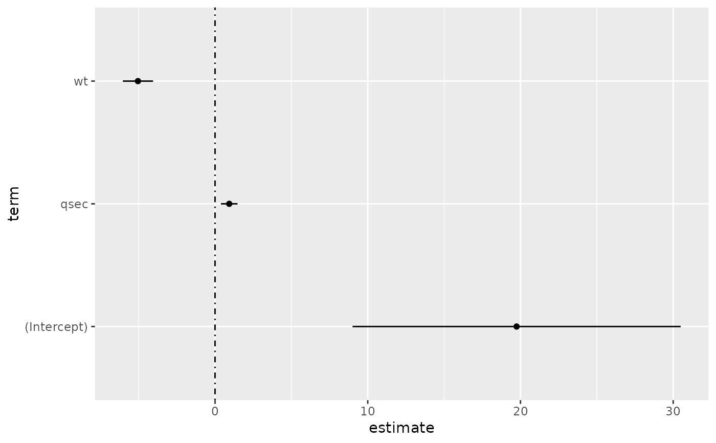
# coefficient plot
d <- tidy(mod, conf.int = TRUE)
ggplot(d, aes(estimate, term, xmin = conf.low, xmax = conf.high, height = 0)) +
geom_point() +
geom_vline(xintercept = 0, lty = 4) +
geom_errorbarh()
 # aside: There are tidy() and glance() methods for lm.summary objects too.
# this can be useful when you want to conserve memory by converting large lm
# objects into their leaner summary.lm equivalents.
s <- summary(mod)
tidy(s, conf.int = TRUE)
#> # A tibble: 3 × 7
#> term estimate std.error statistic p.value conf.low conf.high
#> <chr> <dbl> <dbl> <dbl> <dbl> <dbl> <dbl>
#> 1 (Intercept) 19.7 5.25 3.76 7.65e- 4 9.00 30.5
#> 2 wt -5.05 0.484 -10.4 2.52e-11 -6.04 -4.06
#> 3 qsec 0.929 0.265 3.51 1.50e- 3 0.387 1.47
glance(s)
#> # A tibble: 1 × 8
#> r.squared adj.r.squared sigma statistic p.value df df.residual nobs
#> <dbl> <dbl> <dbl> <dbl> <dbl> <dbl> <int> <dbl>
#> 1 0.826 0.814 2.60 69.0 9.39e-12 2 29 32
augment(mod)
#> # A tibble: 32 × 10
#> .rownames mpg wt qsec .fitted .resid .hat .sigma .cooksd
#> <chr> <dbl> <dbl> <dbl> <dbl> <dbl> <dbl> <dbl> <dbl>
#> 1 Mazda RX4 21 2.62 16.5 21.8 -0.815 0.0693 2.64 2.63e-3
#> 2 Mazda RX4 Wag 21 2.88 17.0 21.0 -0.0482 0.0444 2.64 5.59e-6
#> 3 Datsun 710 22.8 2.32 18.6 25.3 -2.53 0.0607 2.60 2.17e-2
#> 4 Hornet 4 Drive 21.4 3.22 19.4 21.6 -0.181 0.0576 2.64 1.05e-4
#> 5 Hornet Sportab… 18.7 3.44 17.0 18.2 0.504 0.0389 2.64 5.29e-4
#> 6 Valiant 18.1 3.46 20.2 21.1 -2.97 0.0957 2.58 5.10e-2
#> 7 Duster 360 14.3 3.57 15.8 16.4 -2.14 0.0729 2.61 1.93e-2
#> 8 Merc 240D 24.4 3.19 20 22.2 2.17 0.0791 2.61 2.18e-2
#> 9 Merc 230 22.8 3.15 22.9 25.1 -2.32 0.295 2.59 1.59e-1
#> 10 Merc 280 19.2 3.44 18.3 19.4 -0.185 0.0358 2.64 6.55e-5
#> # ℹ 22 more rows
#> # ℹ 1 more variable: .std.resid <dbl>
augment(mod, mtcars, interval = "confidence")
#> # A tibble: 32 × 20
#> .rownames mpg cyl disp hp drat wt qsec vs am gear
#> <chr> <dbl> <dbl> <dbl> <dbl> <dbl> <dbl> <dbl> <dbl> <dbl> <dbl>
#> 1 Mazda RX4 21 6 160 110 3.9 2.62 16.5 0 1 4
#> 2 Mazda RX4 … 21 6 160 110 3.9 2.88 17.0 0 1 4
#> 3 Datsun 710 22.8 4 108 93 3.85 2.32 18.6 1 1 4
#> 4 Hornet 4 D… 21.4 6 258 110 3.08 3.22 19.4 1 0 3
#> 5 Hornet Spo… 18.7 8 360 175 3.15 3.44 17.0 0 0 3
#> 6 Valiant 18.1 6 225 105 2.76 3.46 20.2 1 0 3
#> 7 Duster 360 14.3 8 360 245 3.21 3.57 15.8 0 0 3
#> 8 Merc 240D 24.4 4 147. 62 3.69 3.19 20 1 0 4
#> 9 Merc 230 22.8 4 141. 95 3.92 3.15 22.9 1 0 4
#> 10 Merc 280 19.2 6 168. 123 3.92 3.44 18.3 1 0 4
#> # ℹ 22 more rows
#> # ℹ 9 more variables: carb <dbl>, .fitted <dbl>, .lower <dbl>,
#> # .upper <dbl>, .resid <dbl>, .hat <dbl>, .sigma <dbl>, .cooksd <dbl>,
#> # .std.resid <dbl>
# predict on new data
newdata <- mtcars %>%
head(6) %>%
mutate(wt = wt + 1)
augment(mod, newdata = newdata)
#> # A tibble: 6 × 14
#> .rownames mpg cyl disp hp drat wt qsec vs am gear
#> <chr> <dbl> <dbl> <dbl> <dbl> <dbl> <dbl> <dbl> <dbl> <dbl> <dbl>
#> 1 Mazda RX4 21 6 160 110 3.9 3.62 16.5 0 1 4
#> 2 Mazda RX4 W… 21 6 160 110 3.9 3.88 17.0 0 1 4
#> 3 Datsun 710 22.8 4 108 93 3.85 3.32 18.6 1 1 4
#> 4 Hornet 4 Dr… 21.4 6 258 110 3.08 4.22 19.4 1 0 3
#> 5 Hornet Spor… 18.7 8 360 175 3.15 4.44 17.0 0 0 3
#> 6 Valiant 18.1 6 225 105 2.76 4.46 20.2 1 0 3
#> # ℹ 3 more variables: carb <dbl>, .fitted <dbl>, .resid <dbl>
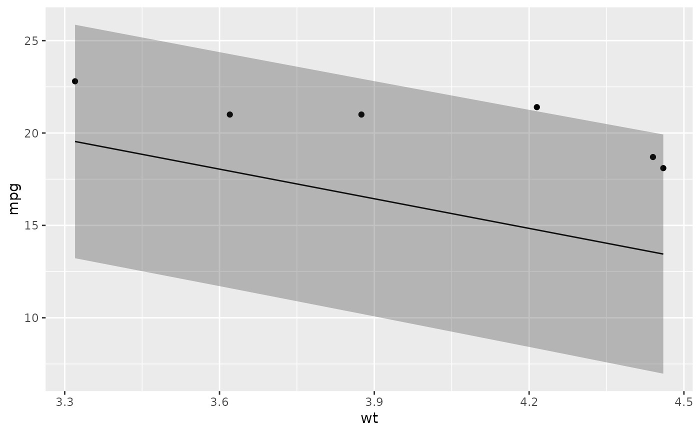
# ggplot2 example where we also construct 95% prediction interval
# simpler bivariate model since we're plotting in 2D
mod2 <- lm(mpg ~ wt, data = mtcars)
au <- augment(mod2, newdata = newdata, interval = "prediction")
ggplot(au, aes(wt, mpg)) +
geom_point() +
geom_line(aes(y = .fitted)) +
geom_ribbon(aes(ymin = .lower, ymax = .upper), col = NA, alpha = 0.3)
# aside: There are tidy() and glance() methods for lm.summary objects too.
# this can be useful when you want to conserve memory by converting large lm
# objects into their leaner summary.lm equivalents.
s <- summary(mod)
tidy(s, conf.int = TRUE)
#> # A tibble: 3 × 7
#> term estimate std.error statistic p.value conf.low conf.high
#> <chr> <dbl> <dbl> <dbl> <dbl> <dbl> <dbl>
#> 1 (Intercept) 19.7 5.25 3.76 7.65e- 4 9.00 30.5
#> 2 wt -5.05 0.484 -10.4 2.52e-11 -6.04 -4.06
#> 3 qsec 0.929 0.265 3.51 1.50e- 3 0.387 1.47
glance(s)
#> # A tibble: 1 × 8
#> r.squared adj.r.squared sigma statistic p.value df df.residual nobs
#> <dbl> <dbl> <dbl> <dbl> <dbl> <dbl> <int> <dbl>
#> 1 0.826 0.814 2.60 69.0 9.39e-12 2 29 32
augment(mod)
#> # A tibble: 32 × 10
#> .rownames mpg wt qsec .fitted .resid .hat .sigma .cooksd
#> <chr> <dbl> <dbl> <dbl> <dbl> <dbl> <dbl> <dbl> <dbl>
#> 1 Mazda RX4 21 2.62 16.5 21.8 -0.815 0.0693 2.64 2.63e-3
#> 2 Mazda RX4 Wag 21 2.88 17.0 21.0 -0.0482 0.0444 2.64 5.59e-6
#> 3 Datsun 710 22.8 2.32 18.6 25.3 -2.53 0.0607 2.60 2.17e-2
#> 4 Hornet 4 Drive 21.4 3.22 19.4 21.6 -0.181 0.0576 2.64 1.05e-4
#> 5 Hornet Sportab… 18.7 3.44 17.0 18.2 0.504 0.0389 2.64 5.29e-4
#> 6 Valiant 18.1 3.46 20.2 21.1 -2.97 0.0957 2.58 5.10e-2
#> 7 Duster 360 14.3 3.57 15.8 16.4 -2.14 0.0729 2.61 1.93e-2
#> 8 Merc 240D 24.4 3.19 20 22.2 2.17 0.0791 2.61 2.18e-2
#> 9 Merc 230 22.8 3.15 22.9 25.1 -2.32 0.295 2.59 1.59e-1
#> 10 Merc 280 19.2 3.44 18.3 19.4 -0.185 0.0358 2.64 6.55e-5
#> # ℹ 22 more rows
#> # ℹ 1 more variable: .std.resid <dbl>
augment(mod, mtcars, interval = "confidence")
#> # A tibble: 32 × 20
#> .rownames mpg cyl disp hp drat wt qsec vs am gear
#> <chr> <dbl> <dbl> <dbl> <dbl> <dbl> <dbl> <dbl> <dbl> <dbl> <dbl>
#> 1 Mazda RX4 21 6 160 110 3.9 2.62 16.5 0 1 4
#> 2 Mazda RX4 … 21 6 160 110 3.9 2.88 17.0 0 1 4
#> 3 Datsun 710 22.8 4 108 93 3.85 2.32 18.6 1 1 4
#> 4 Hornet 4 D… 21.4 6 258 110 3.08 3.22 19.4 1 0 3
#> 5 Hornet Spo… 18.7 8 360 175 3.15 3.44 17.0 0 0 3
#> 6 Valiant 18.1 6 225 105 2.76 3.46 20.2 1 0 3
#> 7 Duster 360 14.3 8 360 245 3.21 3.57 15.8 0 0 3
#> 8 Merc 240D 24.4 4 147. 62 3.69 3.19 20 1 0 4
#> 9 Merc 230 22.8 4 141. 95 3.92 3.15 22.9 1 0 4
#> 10 Merc 280 19.2 6 168. 123 3.92 3.44 18.3 1 0 4
#> # ℹ 22 more rows
#> # ℹ 9 more variables: carb <dbl>, .fitted <dbl>, .lower <dbl>,
#> # .upper <dbl>, .resid <dbl>, .hat <dbl>, .sigma <dbl>, .cooksd <dbl>,
#> # .std.resid <dbl>
# predict on new data
newdata <- mtcars %>%
head(6) %>%
mutate(wt = wt + 1)
augment(mod, newdata = newdata)
#> # A tibble: 6 × 14
#> .rownames mpg cyl disp hp drat wt qsec vs am gear
#> <chr> <dbl> <dbl> <dbl> <dbl> <dbl> <dbl> <dbl> <dbl> <dbl> <dbl>
#> 1 Mazda RX4 21 6 160 110 3.9 3.62 16.5 0 1 4
#> 2 Mazda RX4 W… 21 6 160 110 3.9 3.88 17.0 0 1 4
#> 3 Datsun 710 22.8 4 108 93 3.85 3.32 18.6 1 1 4
#> 4 Hornet 4 Dr… 21.4 6 258 110 3.08 4.22 19.4 1 0 3
#> 5 Hornet Spor… 18.7 8 360 175 3.15 4.44 17.0 0 0 3
#> 6 Valiant 18.1 6 225 105 2.76 4.46 20.2 1 0 3
#> # ℹ 3 more variables: carb <dbl>, .fitted <dbl>, .resid <dbl>
# ggplot2 example where we also construct 95% prediction interval
# simpler bivariate model since we're plotting in 2D
mod2 <- lm(mpg ~ wt, data = mtcars)
au <- augment(mod2, newdata = newdata, interval = "prediction")
ggplot(au, aes(wt, mpg)) +
geom_point() +
geom_line(aes(y = .fitted)) +
geom_ribbon(aes(ymin = .lower, ymax = .upper), col = NA, alpha = 0.3)
 # predict on new data without outcome variable. Output does not include .resid
newdata <- newdata %>%
select(-mpg)
augment(mod, newdata = newdata)
#> # A tibble: 6 × 12
#> .rownames cyl disp hp drat wt qsec vs am gear carb
#> <chr> <dbl> <dbl> <dbl> <dbl> <dbl> <dbl> <dbl> <dbl> <dbl> <dbl>
#> 1 Mazda RX4 6 160 110 3.9 3.62 16.5 0 1 4 4
#> 2 Mazda RX4 W… 6 160 110 3.9 3.88 17.0 0 1 4 4
#> 3 Datsun 710 4 108 93 3.85 3.32 18.6 1 1 4 1
#> 4 Hornet 4 Dr… 6 258 110 3.08 4.22 19.4 1 0 3 1
#> 5 Hornet Spor… 8 360 175 3.15 4.44 17.0 0 0 3 2
#> 6 Valiant 6 225 105 2.76 4.46 20.2 1 0 3 1
#> # ℹ 1 more variable: .fitted <dbl>
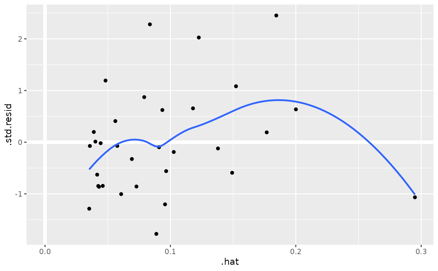
au <- augment(mod, data = mtcars)
ggplot(au, aes(.hat, .std.resid)) +
geom_vline(size = 2, colour = "white", xintercept = 0) +
geom_hline(size = 2, colour = "white", yintercept = 0) +
geom_point() +
geom_smooth(se = FALSE)
#> `geom_smooth()` using method = 'loess' and formula = 'y ~ x'
# predict on new data without outcome variable. Output does not include .resid
newdata <- newdata %>%
select(-mpg)
augment(mod, newdata = newdata)
#> # A tibble: 6 × 12
#> .rownames cyl disp hp drat wt qsec vs am gear carb
#> <chr> <dbl> <dbl> <dbl> <dbl> <dbl> <dbl> <dbl> <dbl> <dbl> <dbl>
#> 1 Mazda RX4 6 160 110 3.9 3.62 16.5 0 1 4 4
#> 2 Mazda RX4 W… 6 160 110 3.9 3.88 17.0 0 1 4 4
#> 3 Datsun 710 4 108 93 3.85 3.32 18.6 1 1 4 1
#> 4 Hornet 4 Dr… 6 258 110 3.08 4.22 19.4 1 0 3 1
#> 5 Hornet Spor… 8 360 175 3.15 4.44 17.0 0 0 3 2
#> 6 Valiant 6 225 105 2.76 4.46 20.2 1 0 3 1
#> # ℹ 1 more variable: .fitted <dbl>
au <- augment(mod, data = mtcars)
ggplot(au, aes(.hat, .std.resid)) +
geom_vline(size = 2, colour = "white", xintercept = 0) +
geom_hline(size = 2, colour = "white", yintercept = 0) +
geom_point() +
geom_smooth(se = FALSE)
#> `geom_smooth()` using method = 'loess' and formula = 'y ~ x'
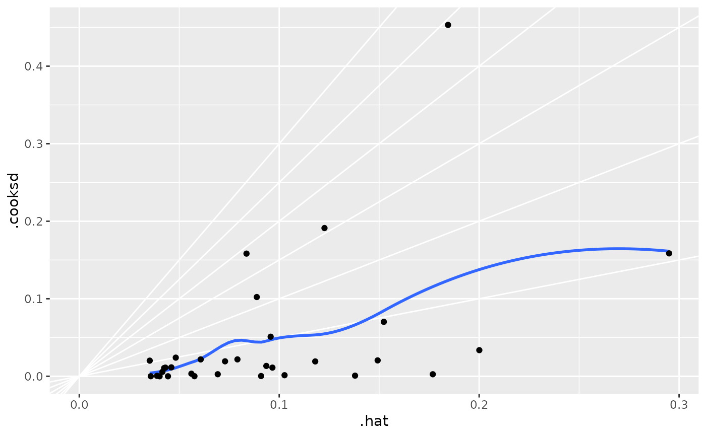
 plot(mod, which = 6)
 ggplot(au, aes(.hat, .cooksd)) +
geom_vline(xintercept = 0, colour = NA) +
geom_abline(slope = seq(0, 3, by = 0.5), colour = "white") +
geom_smooth(se = FALSE) +
geom_point()
#> `geom_smooth()` using method = 'loess' and formula = 'y ~ x'
ggplot(au, aes(.hat, .cooksd)) +
geom_vline(xintercept = 0, colour = NA) +
geom_abline(slope = seq(0, 3, by = 0.5), colour = "white") +
geom_smooth(se = FALSE) +
geom_point()
#> `geom_smooth()` using method = 'loess' and formula = 'y ~ x'
 # column-wise models
a <- matrix(rnorm(20), nrow = 10)
b <- a + rnorm(length(a))
result <- lm(b ~ a)
tidy(result)
#> # A tibble: 6 × 6
#> response term estimate std.error statistic p.value
#> <chr> <chr> <dbl> <dbl> <dbl> <dbl>
#> 1 Y1 (Intercept) 0.591 0.359 1.64 0.144
#> 2 Y1 a1 0.971 0.284 3.42 0.0111
#> 3 Y1 a2 -0.0905 0.414 -0.219 0.833
#> 4 Y2 (Intercept) 0.0105 0.350 0.0299 0.977
#> 5 Y2 a1 0.00789 0.277 0.0285 0.978
#> 6 Y2 a2 1.90 0.403 4.72 0.00216
# column-wise models
a <- matrix(rnorm(20), nrow = 10)
b <- a + rnorm(length(a))
result <- lm(b ~ a)
tidy(result)
#> # A tibble: 6 × 6
#> response term estimate std.error statistic p.value
#> <chr> <chr> <dbl> <dbl> <dbl> <dbl>
#> 1 Y1 (Intercept) 0.591 0.359 1.64 0.144
#> 2 Y1 a1 0.971 0.284 3.42 0.0111
#> 3 Y1 a2 -0.0905 0.414 -0.219 0.833
#> 4 Y2 (Intercept) 0.0105 0.350 0.0299 0.977
#> 5 Y2 a1 0.00789 0.277 0.0285 0.978
#> 6 Y2 a2 1.90 0.403 4.72 0.00216
相关用法
- R broom glance.lmRob 看一眼 lmRob 对象
- R broom glance.lmodel2 浏览 a(n) lmodel2 对象
- R broom glance.lavaan 瞥一眼熔岩物体
- R broom glance.rlm 浏览 a(n) rlm 对象
- R broom glance.felm 瞥一眼毛毡物体
- R broom glance.geeglm 浏览 a(n) geeglm 对象
- R broom glance.plm 浏览一个 (n) plm 对象
- R broom glance.biglm 浏览 a(n) biglm 对象
- R broom glance.clm 浏览 a(n) clm 对象
- R broom glance.rma 浏览一个(n) rma 对象
- R broom glance.multinom 浏览一个(n)多项对象
- R broom glance.survexp 浏览 a(n) survexp 对象
- R broom glance.survreg 看一眼 survreg 对象
- R broom glance.rq 查看 a(n) rq 对象
- R broom glance.mjoint 查看 a(n) mjoint 对象
- R broom glance.fitdistr 浏览 a(n) fitdistr 对象
- R broom glance.glm 浏览 a(n) glm 对象
- R broom glance.coxph 浏览 a(n) coxph 对象
- R broom glance.margins 浏览 (n) 个 margins 对象
- R broom glance.poLCA 浏览一个(n) poLCA 对象
- R broom glance.aov 瞥一眼 lm 物体
- R broom glance.sarlm 浏览一个(n)spatialreg对象
- R broom glance.polr 浏览 a(n) polr 对象
- R broom glance.negbin 看一眼 negbin 对象
- R broom glance.mlogit 浏览一个(n) mlogit 对象
注:本文由纯净天空筛选整理自等大神的英文原创作品 Glance at a(n) lm object。非经特殊声明,原始代码版权归原作者所有,本译文未经允许或授权,请勿转载或复制。