Glance 接受模型对象并返回 tibble::tibble(),其中仅包含一行模型摘要。摘要通常是拟合优度度量、残差假设检验的 p 值或模型收敛信息。
Glance 永远不会返返回自对建模函数的原始调用的信息。这包括建模函数的名称或传递给建模函数的任何参数。
Glance 不计算汇总度量。相反,它将这些计算外包给适当的方法并将结果收集在一起。有时拟合优度测量是不确定的。在这些情况下,该度量将报告为 NA 。
无论模型矩阵是否秩亏,Glance 都会返回相同的列数。如果是这样,则不再具有明确定义值的列中的条目将使用适当类型的 NA 进行填充。
参数
- x
-
lmodel2::lmodel2()返回的lmodel2对象。 - ...
-
附加参数。不曾用过。仅需要匹配通用签名。注意:拼写错误的参数将被吸收到
...中,并被忽略。如果拼写错误的参数有默认值,则将使用默认值。例如,如果您传递conf.lvel = 0.9,所有计算将使用conf.level = 0.95进行。这里有两个异常:
也可以看看
其他 lmodel2 整理器:tidy.lmodel2()
值
恰好只有一行和一列的 tibble::tibble():
- nobs
-
使用的观察数。
- p.value
-
对应于检验统计量的 P 值。
- r.squared
-
R 平方统计量,或模型解释的变异百分比。也称为决定系数。
- theta
-
OLS 线 `lm(y ~ x)` 和 `lm(x ~ y)` 之间的角度
- H
-
用于计算长轴斜率置信区间的 H 统计量
例子
# load libraries for models and data
library(lmodel2)
data(mod2ex2)
Ex2.res <- lmodel2(Prey ~ Predators, data = mod2ex2, "relative", "relative", 99)
Ex2.res
#>
#> Model II regression
#>
#> Call: lmodel2(formula = Prey ~ Predators, data = mod2ex2, range.y
#> = "relative", range.x = "relative", nperm = 99)
#>
#> n = 20 r = 0.8600787 r-square = 0.7397354
#> Parametric P-values: 2-tailed = 1.161748e-06 1-tailed = 5.808741e-07
#> Angle between the two OLS regression lines = 5.106227 degrees
#>
#> Permutation tests of OLS, MA, RMA slopes: 1-tailed, tail corresponding to sign
#> A permutation test of r is equivalent to a permutation test of the OLS slope
#> P-perm for SMA = NA because the SMA slope cannot be tested
#>
#> Regression results
#> Method Intercept Slope Angle (degrees) P-perm (1-tailed)
#> 1 OLS 20.02675 2.631527 69.19283 0.01
#> 2 MA 13.05968 3.465907 73.90584 0.01
#> 3 SMA 16.45205 3.059635 71.90073 NA
#> 4 RMA 17.25651 2.963292 71.35239 0.01
#>
#> Confidence intervals
#> Method 2.5%-Intercept 97.5%-Intercept 2.5%-Slope 97.5%-Slope
#> 1 OLS 12.490993 27.56251 1.858578 3.404476
#> 2 MA 1.347422 19.76310 2.663101 4.868572
#> 3 SMA 9.195287 22.10353 2.382810 3.928708
#> 4 RMA 8.962997 23.84493 2.174260 3.956527
#>
#> Eigenvalues: 269.8212 6.418234
#>
#> H statistic used for computing C.I. of MA: 0.006120651
#>
# summarize model fit with tidiers + visualization
tidy(Ex2.res)
#> # A tibble: 8 × 6
#> method term estimate conf.low conf.high p.value
#> <chr> <chr> <dbl> <dbl> <dbl> <dbl>
#> 1 MA Intercept 13.1 1.35 19.8 0.01
#> 2 MA Slope 3.47 2.66 4.87 0.01
#> 3 OLS Intercept 20.0 12.5 27.6 0.01
#> 4 OLS Slope 2.63 1.86 3.40 0.01
#> 5 RMA Intercept 17.3 8.96 23.8 0.01
#> 6 RMA Slope 2.96 2.17 3.96 0.01
#> 7 SMA Intercept 16.5 9.20 22.1 NA
#> 8 SMA Slope 3.06 2.38 3.93 NA
glance(Ex2.res)
#> # A tibble: 1 × 5
#> r.squared theta p.value H nobs
#> <dbl> <dbl> <dbl> <dbl> <int>
#> 1 0.740 5.11 0.00000116 0.00612 20
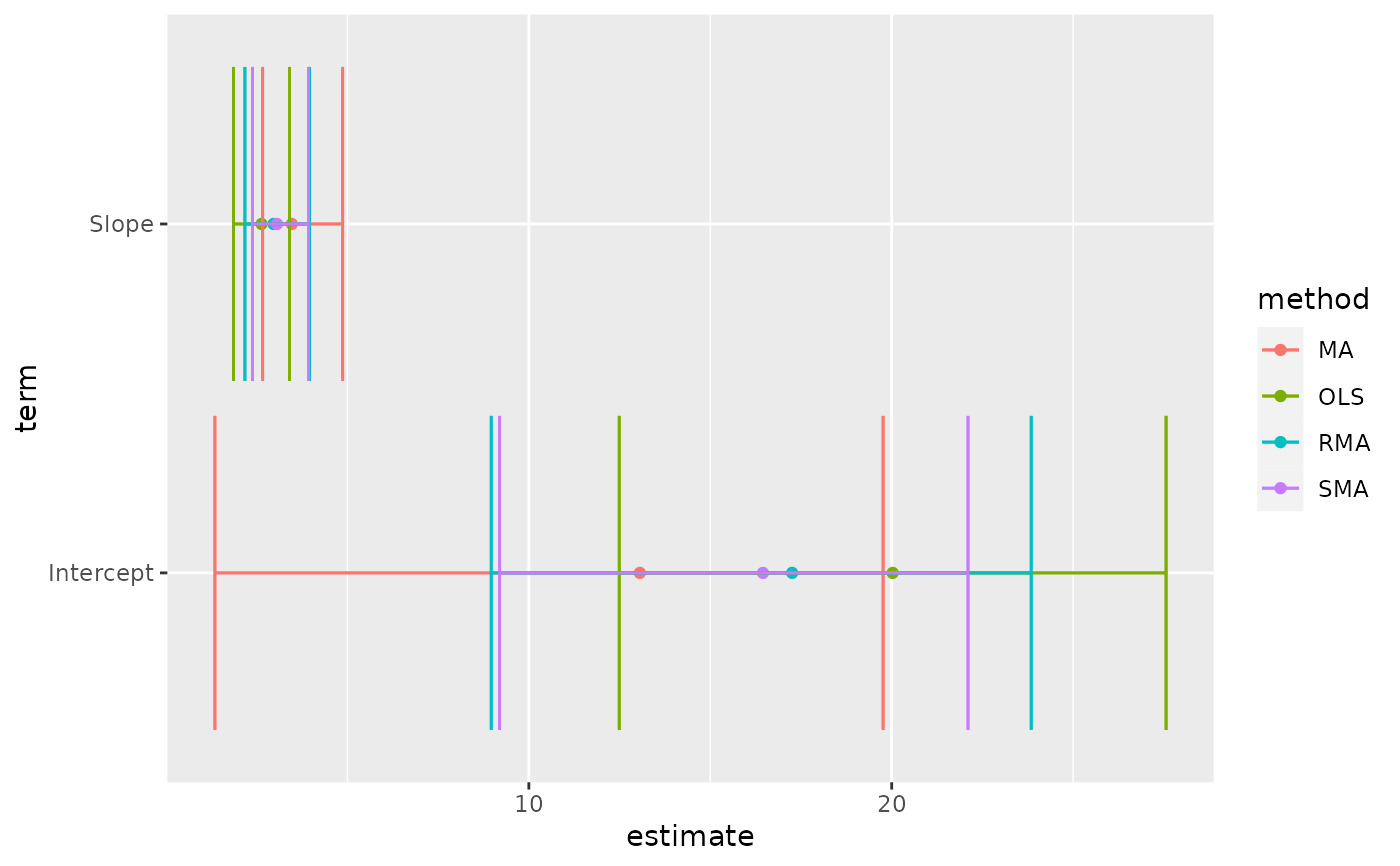
# this allows coefficient plots with ggplot2
library(ggplot2)
ggplot(tidy(Ex2.res), aes(estimate, term, color = method)) +
geom_point() +
geom_errorbarh(aes(xmin = conf.low, xmax = conf.high)) +
geom_errorbarh(aes(xmin = conf.low, xmax = conf.high))
相关用法
- R broom glance.lmRob 看一眼 lmRob 对象
- R broom glance.lm 瞥一眼 lm 物体
- R broom glance.lavaan 瞥一眼熔岩物体
- R broom glance.rlm 浏览 a(n) rlm 对象
- R broom glance.felm 瞥一眼毛毡物体
- R broom glance.geeglm 浏览 a(n) geeglm 对象
- R broom glance.plm 浏览一个 (n) plm 对象
- R broom glance.biglm 浏览 a(n) biglm 对象
- R broom glance.clm 浏览 a(n) clm 对象
- R broom glance.rma 浏览一个(n) rma 对象
- R broom glance.multinom 浏览一个(n)多项对象
- R broom glance.survexp 浏览 a(n) survexp 对象
- R broom glance.survreg 看一眼 survreg 对象
- R broom glance.rq 查看 a(n) rq 对象
- R broom glance.mjoint 查看 a(n) mjoint 对象
- R broom glance.fitdistr 浏览 a(n) fitdistr 对象
- R broom glance.glm 浏览 a(n) glm 对象
- R broom glance.coxph 浏览 a(n) coxph 对象
- R broom glance.margins 浏览 (n) 个 margins 对象
- R broom glance.poLCA 浏览一个(n) poLCA 对象
- R broom glance.aov 瞥一眼 lm 物体
- R broom glance.sarlm 浏览一个(n)spatialreg对象
- R broom glance.polr 浏览 a(n) polr 对象
- R broom glance.negbin 看一眼 negbin 对象
- R broom glance.mlogit 浏览一个(n) mlogit 对象
注:本文由纯净天空筛选整理自等大神的英文原创作品 Glance at a(n) lmodel2 object。非经特殊声明,原始代码版权归原作者所有,本译文未经允许或授权,请勿转载或复制。