Python SciPy special.tklmbda用法及代碼示例

本文簡要介紹 python 語言中 scipy.special.tklmbda 的用法。

用法:

scipy.special.tklmbda(x, lmbda, out=None) = <ufunc 'tklmbda'>#

Tukey lambda 分布的累積分布函數。

參數 ：：

x, lmbda： array_like

參數

out： ndarray，可選

函數結果的可選輸出數組

返回 ：：

cdf： 標量或 ndarray

Tukey lambda CDF 的值

例子：

>>> import numpy as np
>>> import matplotlib.pyplot as plt
>>> from scipy.special import tklmbda, expit

計算 lmbda = -1.5 時多個 x 值處的 Tukey lambda 分布的累積分布函數 (CDF)。

>>> x = np.linspace(-2, 2, 9)
>>> x
array([-2. , -1.5, -1. , -0.5,  0. ,  0.5,  1. ,  1.5,  2. ])
>>> tklmbda(x, -1.5)
array([0.34688734, 0.3786554 , 0.41528805, 0.45629737, 0.5       ,
       0.54370263, 0.58471195, 0.6213446 , 0.65311266])

當 lmbda 為0時，該函數為logistic sigmoid函數，在 scipy.special 中實現為 expit 。

>>> tklmbda(x, 0)
array([0.11920292, 0.18242552, 0.26894142, 0.37754067, 0.5       ,
       0.62245933, 0.73105858, 0.81757448, 0.88079708])
>>> expit(x)
array([0.11920292, 0.18242552, 0.26894142, 0.37754067, 0.5       ,
       0.62245933, 0.73105858, 0.81757448, 0.88079708])

當 lmbda 為1時，Tukey lambda分布在區間[-1, 1]上是均勻的，因此CDF線性增加。

>>> t = np.linspace(-1, 1, 9)
>>> tklmbda(t, 1)
array([0.   , 0.125, 0.25 , 0.375, 0.5  , 0.625, 0.75 , 0.875, 1.   ])

接下來，我們為 lmbda 的多個值生成圖。

第一張圖顯示了 lmbda <= 0 的圖表。

>>> styles = ['-', '-.', '--', ':']
>>> fig, ax = plt.subplots()
>>> x = np.linspace(-12, 12, 500)
>>> for k, lmbda in enumerate([-1.0, -0.5, 0.0]):
...     y = tklmbda(x, lmbda)
...     ax.plot(x, y, styles[k], label=f'$\lambda$ = {lmbda:-4.1f}')

>>> ax.set_title('tklmbda(x, $\lambda$)')
>>> ax.set_label('x')
>>> ax.legend(framealpha=1, shadow=True)
>>> ax.grid(True)

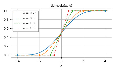
第二張圖顯示了 lmbda > 0 的圖表。圖表中的點顯示了分布的支持範圍。

>>> fig, ax = plt.subplots()
>>> x = np.linspace(-4.2, 4.2, 500)
>>> lmbdas = [0.25, 0.5, 1.0, 1.5]
>>> for k, lmbda in enumerate(lmbdas):
...     y = tklmbda(x, lmbda)
...     ax.plot(x, y, styles[k], label=f'$\lambda$ = {lmbda}')

>>> ax.set_prop_cycle(None)
>>> for lmbda in lmbdas:
...     ax.plot([-1/lmbda, 1/lmbda], [0, 1], '.', ms=8)

>>> ax.set_title('tklmbda(x, $\lambda$)')
>>> ax.set_xlabel('x')
>>> ax.legend(framealpha=1, shadow=True)
>>> ax.grid(True)

>>> plt.tight_layout()
>>> plt.show()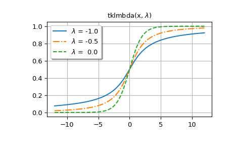

Tukey lambda 分布的 CDF 也實現為 scipy.stats.tukeylambda 的 cdf 方法。在下文中，tukeylambda.cdf(x, -0.5) 和 tklmbda(x, -0.5) 計算相同的值：

>>> from scipy.stats import tukeylambda
>>> x = np.linspace(-2, 2, 9)

>>> tukeylambda.cdf(x, -0.5)
array([0.21995157, 0.27093858, 0.33541677, 0.41328161, 0.5       ,
       0.58671839, 0.66458323, 0.72906142, 0.78004843])

>>> tklmbda(x, -0.5)
array([0.21995157, 0.27093858, 0.33541677, 0.41328161, 0.5       ,
       0.58671839, 0.66458323, 0.72906142, 0.78004843])

tukeylambda 中的實現還提供位置和尺度參數，以及其他方法，例如 pdf()(概率密度函數)和 ppf()(CDF 的逆函數)，因此對於使用 Tukey lambda 分布，tukeylambda 更普遍有用。 tklmbda 的主要優點是它比 tukeylambda.cdf 快得多。