Python SciPy special.fdtrc用法及代碼示例

本文簡要介紹 python 語言中 scipy.special.fdtrc 的用法。

用法:

scipy.special.fdtrc(dfn, dfd, x, out=None) = <ufunc 'fdtrc'>#

F 生存函數。

返回補集的 F-distribution 函數(密度的積分x到無窮遠)。

參數 ：：

dfn： array_like

第一個參數(正浮點數)。

dfd： array_like

第二個參數(正浮點數)。

x： array_like

參數(非負浮點數)。

out： ndarray，可選

函數值的可選輸出數組

返回 ：：

y： 標量或 ndarray

補充的 F-distribution 函數在 x 處帶有參數 dfn 和 dfd。

注意：

采用正則化不完全beta函數，根據公式，

\[F(d_n, d_d; x) = I_{d_d/(d_d + xd_n)}(d_d/2, d_n/2).\]

Cephes [1] 例程的包裝器 fdtrc 。 F 分布也可用作 scipy.stats.f 。與 scipy.stats.f 的 sf 方法相比，直接調用 fdtrc 可以提高性能(請參見下麵的最後一個示例)。

參考：

[1]

Cephes 數學函數庫，http://www.netlib.org/cephes/

例子：

計算 x=1 處的 dfn=1 和 dfd=2 的函數。

>>> import numpy as np
>>> from scipy.special import fdtrc
>>> fdtrc(1, 2, 1)
0.42264973081037427

通過為 x 提供 NumPy 數組來計算多個點的函數。

>>> x = np.array([0.5, 2., 3.])
>>> fdtrc(1, 2, x)
array([0.5527864 , 0.29289322, 0.22540333])

繪製多個參數集的函數。

>>> import matplotlib.pyplot as plt
>>> dfn_parameters = [1, 5, 10, 50]
>>> dfd_parameters = [1, 1, 2, 3]
>>> linestyles = ['solid', 'dashed', 'dotted', 'dashdot']
>>> parameters_list = list(zip(dfn_parameters, dfd_parameters,
...                            linestyles))
>>> x = np.linspace(0, 30, 1000)
>>> fig, ax = plt.subplots()
>>> for parameter_set in parameters_list:
...     dfn, dfd, style = parameter_set
...     fdtrc_vals = fdtrc(dfn, dfd, x)
...     ax.plot(x, fdtrc_vals, label=rf"$d_n={dfn},\, d_d={dfd}$",
...             ls=style)
>>> ax.legend()
>>> ax.set_xlabel("$x$")
>>> ax.set_title("F distribution survival function")
>>> plt.show()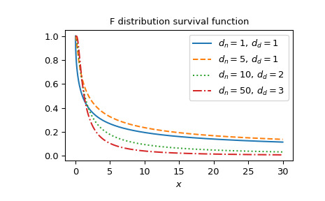

F 分布也可用作 scipy.stats.f 。直接使用 fdtrc 比調用 scipy.stats.f 的 sf 方法要快得多，特別是對於小型數組或單個值。為了獲得相同的結果，必須使用以下參數化：stats.f(dfn, dfd).sf(x)=fdtrc(dfn, dfd, x)。

>>> from scipy.stats import f
>>> dfn, dfd = 1, 2
>>> x = 1
>>> fdtrc_res = fdtrc(dfn, dfd, x)  # this will often be faster than below
>>> f_dist_res = f(dfn, dfd).sf(x)
>>> f_dist_res == fdtrc_res  # test that results are equal
True