R ggplot2 facet_wrap 将 1d 面板带包成 2d 面板

facet_wrap(
  facets,
  nrow = NULL,
  ncol = NULL,
  scales = "fixed",
  shrink = TRUE,
  labeller = "label_value",
  as.table = TRUE,
  switch = deprecated(),
  drop = TRUE,
  dir = "h",
  strip.position = "top"
)

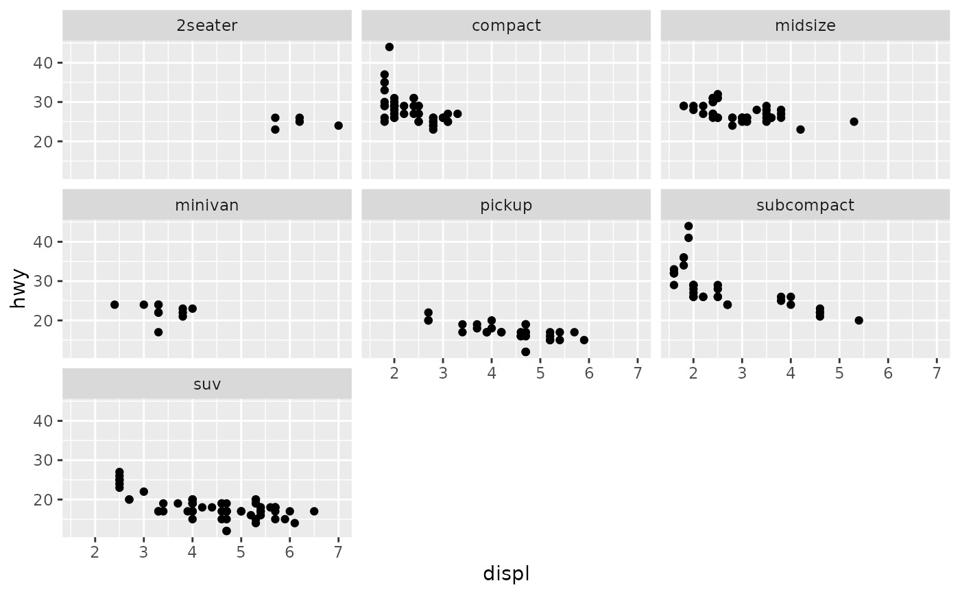
p <- ggplot(mpg, aes(displ, hwy)) + geom_point()

# Use vars() to supply faceting variables:
p + facet_wrap(vars(class))


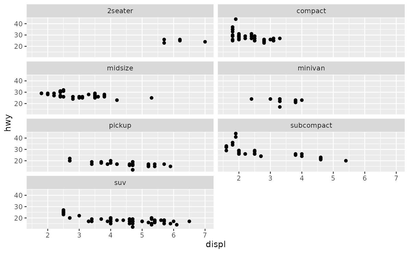
# Control the number of rows and columns with nrow and ncol
p + facet_wrap(vars(class), nrow = 4)


# \donttest{
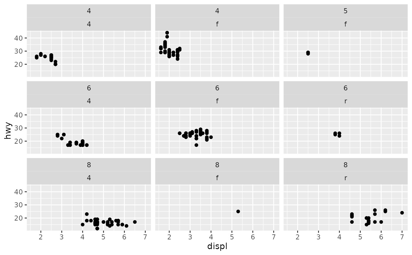
# You can facet by multiple variables
ggplot(mpg, aes(displ, hwy)) +
  geom_point() +
  facet_wrap(vars(cyl, drv))


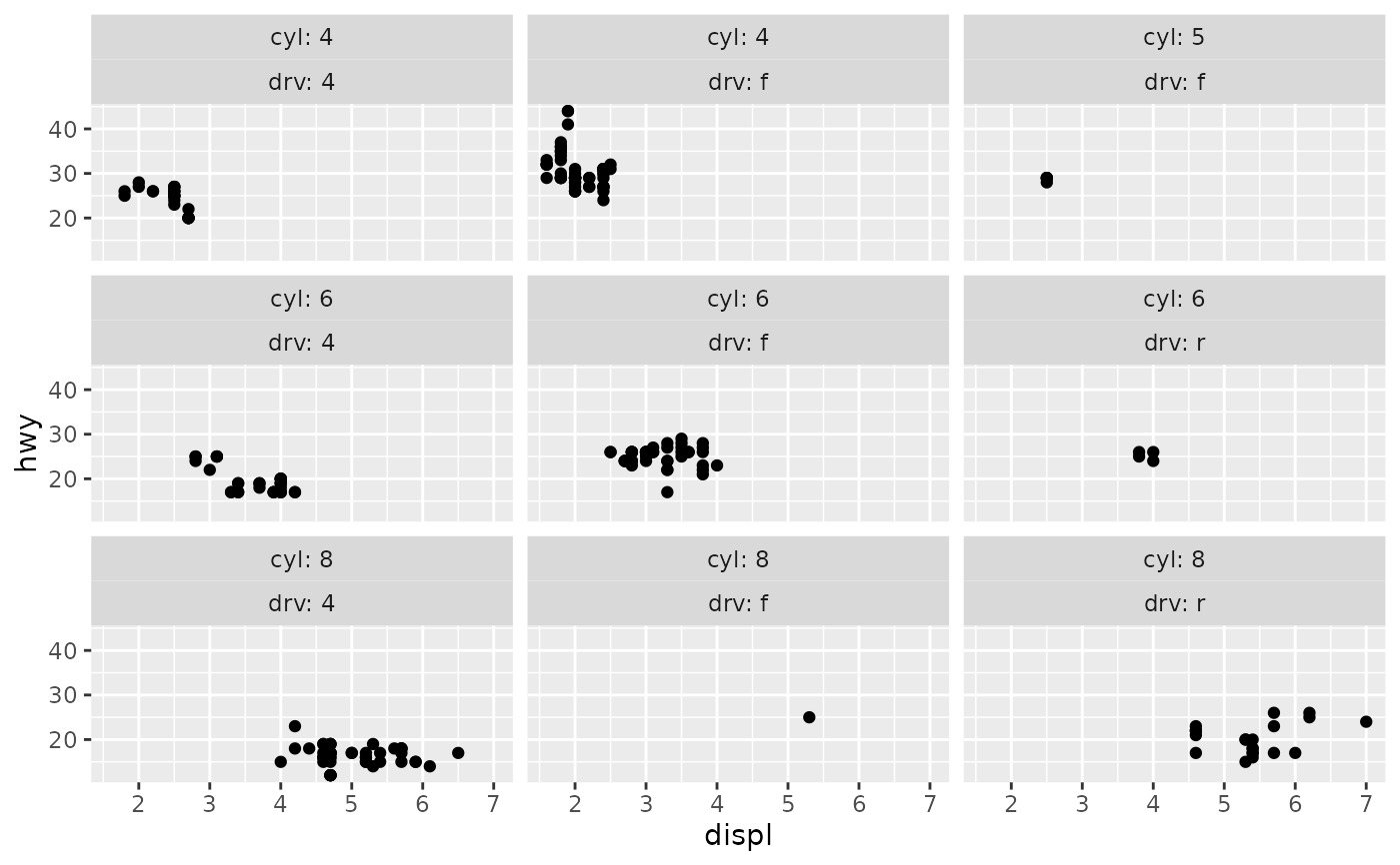
# Use the `labeller` option to control how labels are printed:
ggplot(mpg, aes(displ, hwy)) +
  geom_point() +
  facet_wrap(vars(cyl, drv), labeller = "label_both")


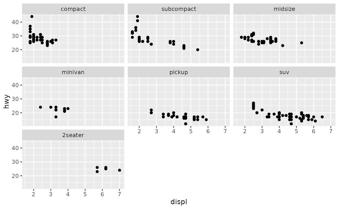
# To change the order in which the panels appear, change the levels
# of the underlying factor.
mpg$class2 <- reorder(mpg$class, mpg$displ)
ggplot(mpg, aes(displ, hwy)) +
  geom_point() +
  facet_wrap(vars(class2))


# By default, the same scales are used for all panels. You can allow
# scales to vary across the panels with the `scales` argument.
# Free scales make it easier to see patterns within each panel, but
# harder to compare across panels.
ggplot(mpg, aes(displ, hwy)) +
  geom_point() +
  facet_wrap(vars(class), scales = "free")


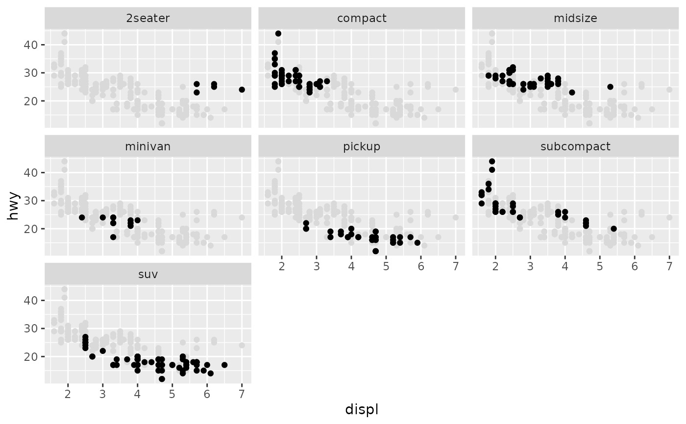
# To repeat the same data in every panel, simply construct a data frame
# that does not contain the faceting variable.
ggplot(mpg, aes(displ, hwy)) +
  geom_point(data = transform(mpg, class = NULL), colour = "grey85") +
  geom_point() +
  facet_wrap(vars(class))


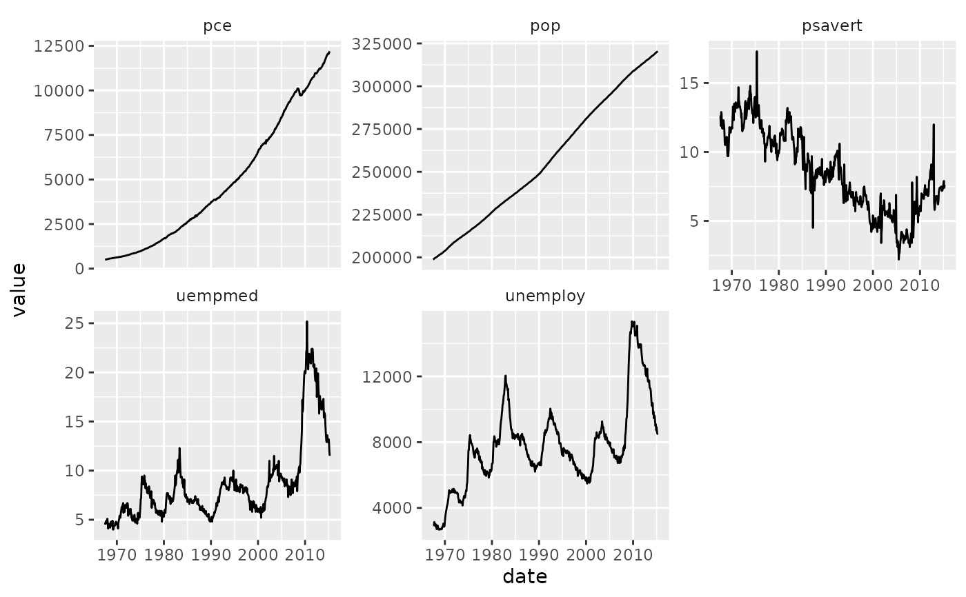
# Use `strip.position` to display the facet labels at the side of your
# choice. Setting it to `bottom` makes it act as a subtitle for the axis.
# This is typically used with free scales and a theme without boxes around
# strip labels.
ggplot(economics_long, aes(date, value)) +
  geom_line() +
  facet_wrap(vars(variable), scales = "free_y", nrow = 2, strip.position = "top") +
  theme(strip.background = element_blank(), strip.placement = "outside")

# }