本文简要介绍 python 语言中 scipy.stats.halflogistic 的用法。
用法:
scipy.stats.halflogistic = <scipy.stats._continuous_distns.halflogistic_gen object>#half-logistic 连续随机变量。
作为
rv_continuous类的实例,halflogistic对象从它继承了一组通用方法(完整列表见下文),并用特定于此特定发行版的详细信息来完成它们。注意:
halflogistic的概率密度函数为:对于 。
上面的概率密度在“standardized” 表格中定义。要移动和/或缩放分布,请使用
loc和scale参数。具体来说,halflogistic.pdf(x, loc, scale)等同于halflogistic.pdf(y) / scale和y = (x - loc) / scale。请注意,移动分布的位置不会使其成为“noncentral” 分布;某些分布的非中心概括可在单独的类中获得。参考:
[1]阿斯加尔扎德等人 (2011)。 “Half-Logistic 分布估计方法的比较”。塞尔丘克·J·阿普尔。数学。 93-108。
例子:
>>> import numpy as np
>>> from scipy.stats import halflogistic
>>> import matplotlib.pyplot as plt
>>> fig, ax = plt.subplots(1, 1)
计算前四个时刻:
>>> mean, var, skew, kurt = halflogistic.stats(moments='mvsk')显示概率密度函数(
pdf):>>> x = np.linspace(halflogistic.ppf(0.01), ... halflogistic.ppf(0.99), 100) >>> ax.plot(x, halflogistic.pdf(x), ... 'r-', lw=5, alpha=0.6, label='halflogistic pdf')或者,可以调用分布对象(作为函数)来固定形状、位置和比例参数。这将返回一个 “frozen” RV 对象,其中包含固定的给定参数。
冻结分布并显示冻结的
pdf:>>> rv = halflogistic() >>> ax.plot(x, rv.pdf(x), 'k-', lw=2, label='frozen pdf')检查
cdf和ppf的准确性:>>> vals = halflogistic.ppf([0.001, 0.5, 0.999]) >>> np.allclose([0.001, 0.5, 0.999], halflogistic.cdf(vals)) True生成随机数:
>>> r = halflogistic.rvs(size=1000)并比较直方图:
>>> ax.hist(r, density=True, bins='auto', histtype='stepfilled', alpha=0.2)
>>> ax.set_xlim([x[0], x[-1]])
>>> ax.legend(loc='best', frameon=False)
>>> plt.show()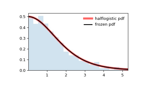
相关用法
- Python SciPy stats.halfnorm用法及代码示例
- Python SciPy stats.halfcauchy用法及代码示例
- Python SciPy stats.halfgennorm用法及代码示例
- Python SciPy stats.hypsecant用法及代码示例
- Python SciPy stats.hmean用法及代码示例
- Python SciPy stats.hypergeom用法及代码示例
- Python SciPy stats.anderson用法及代码示例
- Python SciPy stats.iqr用法及代码示例
- Python SciPy stats.genpareto用法及代码示例
- Python SciPy stats.skewnorm用法及代码示例
- Python SciPy stats.cosine用法及代码示例
- Python SciPy stats.norminvgauss用法及代码示例
- Python SciPy stats.directional_stats用法及代码示例
- Python SciPy stats.invwishart用法及代码示例
- Python SciPy stats.bartlett用法及代码示例
- Python SciPy stats.levy_stable用法及代码示例
- Python SciPy stats.page_trend_test用法及代码示例
- Python SciPy stats.itemfreq用法及代码示例
- Python SciPy stats.exponpow用法及代码示例
- Python SciPy stats.gumbel_l用法及代码示例
- Python SciPy stats.chisquare用法及代码示例
- Python SciPy stats.semicircular用法及代码示例
- Python SciPy stats.gzscore用法及代码示例
- Python SciPy stats.gompertz用法及代码示例
- Python SciPy stats.normaltest用法及代码示例
注:本文由纯净天空筛选整理自scipy.org大神的英文原创作品 scipy.stats.halflogistic。非经特殊声明,原始代码版权归原作者所有,本译文未经允许或授权,请勿转载或复制。