Tidy 总结了有关模型组件的信息。模型组件可能是回归中的单个项、单个假设、聚类或类。 tidy 所认为的模型组件的确切含义因模型而异,但通常是不言而喻的。如果模型具有多种不同类型的组件,您将需要指定要返回哪些组件。
参数
- x
-
stats::prcomp()返回的prcomp对象。 - matrix
-
指定应整理 PCA 的哪个组件的字符。
-
"u"、"samples"、"scores"或"x":返回有关从原始空间到主成分空间的映射的信息。 -
"v"、"rotation"、"loadings"或"variables":将有关从主成分空间映射回原始空间的信息返回。 -
"d"、"eigenvalues"或"pcs":返回有关特征值的信息。
-
- ...
-
附加参数。不曾用过。仅需要匹配通用签名。注意:拼写错误的参数将被吸收到
...中,并被忽略。如果拼写错误的参数有默认值,则将使用默认值。例如,如果您传递conf.lvel = 0.9,所有计算将使用conf.level = 0.95进行。这里有两个异常:
值
tibble::tibble,其列取决于正在整理的 PCA 的组件。
如果 matrix 是 "u" 、 "samples" 、 "scores" 或 "x" ,整理输出中的每一行对应于 PCA 空间中的原始数据。这些列是:
row-
原始观察的 ID(即原始数据中的行名称)。
PC-
表示主成分的整数。
value-
该特定主成分的观察分数。即 PCA 空间中观测的位置。
如果 matrix 是 "v" 、 "rotation" 、 "loadings" 或 "variables" ,则整理输出中的每一行对应于原始空间中主成分的信息。这些列是:
row-
执行 PCA 的数据集的变量标签(列名)。
PC-
指示主成分的整数向量。
value-
指定主成分上的特征向量(轴得分)值。
如果 matrix 是 "d" 、 "eigenvalues" 或 "pcs" ,则列为:
PC-
指示主成分的整数向量。
std.dev-
此 PC 解释的标准偏差。
percent-
该分量解释的变异分数(0 到 1 之间的数值)。
cumulative-
由主要成分解释的累积变异分数,直至该成分(0 到 1 之间的数值)。
细节
有关如何解释各种整理矩阵的信息,请参阅 https://stats.stackexchange.com/questions/134282/relationship-between-svd-and-pca-how-to-use-svd-to-perform-pca。请注意,SVD 仅相当于中心数据上的 PCA。
也可以看看
其他 svd 整理器:augment.prcomp()、tidy_irlba()、tidy_svd()
例子
pc <- prcomp(USArrests, scale = TRUE)
# information about rotation
tidy(pc)
#> # A tibble: 200 × 3
#> row PC value
#> <chr> <dbl> <dbl>
#> 1 Alabama 1 -0.976
#> 2 Alabama 2 -1.12
#> 3 Alabama 3 0.440
#> 4 Alabama 4 0.155
#> 5 Alaska 1 -1.93
#> 6 Alaska 2 -1.06
#> 7 Alaska 3 -2.02
#> 8 Alaska 4 -0.434
#> 9 Arizona 1 -1.75
#> 10 Arizona 2 0.738
#> # ℹ 190 more rows
# information about samples (states)
tidy(pc, "samples")
#> # A tibble: 200 × 3
#> row PC value
#> <chr> <dbl> <dbl>
#> 1 Alabama 1 -0.976
#> 2 Alabama 2 -1.12
#> 3 Alabama 3 0.440
#> 4 Alabama 4 0.155
#> 5 Alaska 1 -1.93
#> 6 Alaska 2 -1.06
#> 7 Alaska 3 -2.02
#> 8 Alaska 4 -0.434
#> 9 Arizona 1 -1.75
#> 10 Arizona 2 0.738
#> # ℹ 190 more rows
# information about PCs
tidy(pc, "pcs")
#> # A tibble: 4 × 4
#> PC std.dev percent cumulative
#> <dbl> <dbl> <dbl> <dbl>
#> 1 1 1.57 0.620 0.620
#> 2 2 0.995 0.247 0.868
#> 3 3 0.597 0.0891 0.957
#> 4 4 0.416 0.0434 1
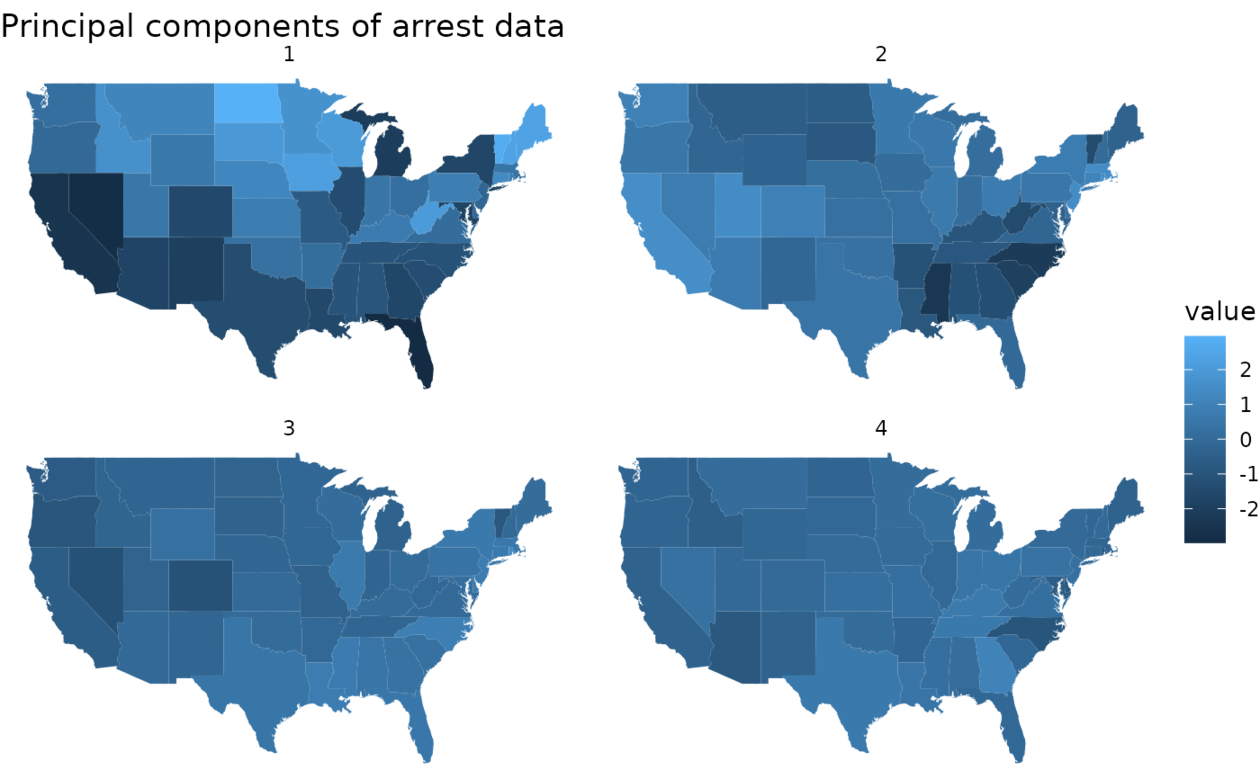
# state map
library(dplyr)
library(ggplot2)
library(maps)
pc %>%
tidy(matrix = "samples") %>%
mutate(region = tolower(row)) %>%
inner_join(map_data("state"), by = "region") %>%
ggplot(aes(long, lat, group = group, fill = value)) +
geom_polygon() +
facet_wrap(~PC) +
theme_void() +
ggtitle("Principal components of arrest data")
#> Warning: Detected an unexpected many-to-many relationship between `x` and `y`.
#> ℹ Row 1 of `x` matches multiple rows in `y`.
#> ℹ Row 1 of `y` matches multiple rows in `x`.
#> ℹ If a many-to-many relationship is expected, set `relationship =
#> "many-to-many"` to silence this warning.
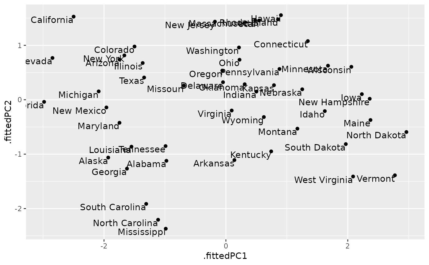
 au <- augment(pc, data = USArrests)
au
#> # A tibble: 50 × 9
#> .rownames Murder Assault UrbanPop Rape .fittedPC1 .fittedPC2
#> <chr> <dbl> <int> <int> <dbl> <dbl> <dbl>
#> 1 Alabama 13.2 236 58 21.2 -0.976 -1.12
#> 2 Alaska 10 263 48 44.5 -1.93 -1.06
#> 3 Arizona 8.1 294 80 31 -1.75 0.738
#> 4 Arkansas 8.8 190 50 19.5 0.140 -1.11
#> 5 California 9 276 91 40.6 -2.50 1.53
#> 6 Colorado 7.9 204 78 38.7 -1.50 0.978
#> 7 Connecticut 3.3 110 77 11.1 1.34 1.08
#> 8 Delaware 5.9 238 72 15.8 -0.0472 0.322
#> 9 Florida 15.4 335 80 31.9 -2.98 -0.0388
#> 10 Georgia 17.4 211 60 25.8 -1.62 -1.27
#> # ℹ 40 more rows
#> # ℹ 2 more variables: .fittedPC3 <dbl>, .fittedPC4 <dbl>
ggplot(au, aes(.fittedPC1, .fittedPC2)) +
geom_point() +
geom_text(aes(label = .rownames), vjust = 1, hjust = 1)
au <- augment(pc, data = USArrests)
au
#> # A tibble: 50 × 9
#> .rownames Murder Assault UrbanPop Rape .fittedPC1 .fittedPC2
#> <chr> <dbl> <int> <int> <dbl> <dbl> <dbl>
#> 1 Alabama 13.2 236 58 21.2 -0.976 -1.12
#> 2 Alaska 10 263 48 44.5 -1.93 -1.06
#> 3 Arizona 8.1 294 80 31 -1.75 0.738
#> 4 Arkansas 8.8 190 50 19.5 0.140 -1.11
#> 5 California 9 276 91 40.6 -2.50 1.53
#> 6 Colorado 7.9 204 78 38.7 -1.50 0.978
#> 7 Connecticut 3.3 110 77 11.1 1.34 1.08
#> 8 Delaware 5.9 238 72 15.8 -0.0472 0.322
#> 9 Florida 15.4 335 80 31.9 -2.98 -0.0388
#> 10 Georgia 17.4 211 60 25.8 -1.62 -1.27
#> # ℹ 40 more rows
#> # ℹ 2 more variables: .fittedPC3 <dbl>, .fittedPC4 <dbl>
ggplot(au, aes(.fittedPC1, .fittedPC2)) +
geom_point() +
geom_text(aes(label = .rownames), vjust = 1, hjust = 1)
相关用法
- R broom tidy.poLCA 整理 a(n) poLCA 对象
- R broom tidy.pairwise.htest 整理 a(n)pairwise.htest 对象
- R broom tidy.polr 整理 a(n) polr 对象
- R broom tidy.pyears 整理 a(n) pyears 对象
- R broom tidy.plm 整理 a(n) plm 对象
- R broom tidy.power.htest 整理 a(n) power.htest 对象
- R broom tidy.pam 整理 a(n) pam 对象
- R broom tidy.robustbase.glmrob 整理 a(n) glmrob 对象
- R broom tidy.acf 整理 a(n) acf 对象
- R broom tidy.robustbase.lmrob 整理 a(n) lmrob 对象
- R broom tidy.biglm 整理 a(n) biglm 对象
- R broom tidy.garch 整理 a(n) garch 对象
- R broom tidy.rq 整理 a(n) rq 对象
- R broom tidy.kmeans 整理 a(n) kmeans 对象
- R broom tidy.betamfx 整理 a(n) betamfx 对象
- R broom tidy.anova 整理 a(n) anova 对象
- R broom tidy.btergm 整理 a(n) btergm 对象
- R broom tidy.cv.glmnet 整理 a(n) cv.glmnet 对象
- R broom tidy.roc 整理 a(n) roc 对象
- R broom tidy.emmGrid 整理 a(n) emmGrid 对象
- R broom tidy.Kendall 整理 a(n) Kendall 对象
- R broom tidy.survreg 整理 a(n) survreg 对象
- R broom tidy.ergm 整理 a(n) ergm 对象
- R broom tidy.coeftest 整理 a(n) coeftest 对象
- R broom tidy.map 整理 a(n) Map对象
注:本文由纯净天空筛选整理自等大神的英文原创作品 Tidy a(n) prcomp object。非经特殊声明,原始代码版权归原作者所有,本译文未经允许或授权,请勿转载或复制。