可視化股票市場結構簡介
本示例采用了幾種無監督學習技術,以從曆史報價的變化中提取股票市場結構。
我們使用的數量是報價的每日變化:關聯報價在一天中往往會一起波動。
下麵是數據分析方法:
學習圖結構
我們使用稀疏逆協方差估計來查找哪些報價跟其他報價條件相關。具體來說,稀疏逆協方差給出了一個圖,即一個連接列表。在圖中對於每個符號(Symbol)來說,它所連接的其他符號可以用來解釋其波動。
聚類
我們使用聚類將表現相似的報價分組在一起。在scikit-learn中可用的各種聚類技術中,我們選用親和力傳播(Affinity Propagation)模型,因為它不強製要求大小相同的簇,並且可以從數據中自動選擇簇數。
請注意,這給了我們與圖不同的表示,因為圖反映了變量之間的條件關係,而聚類反映了邊際屬性:聚類在一起的變量對整個股票市場具有相似的影響。
嵌入2D空間
出於可視化目的,我們需要在2D畫布上布置不同的符號(Symbol)。為此,我們使用流形學習(Manifold learning )技術獲取2D嵌入(Embedding)。
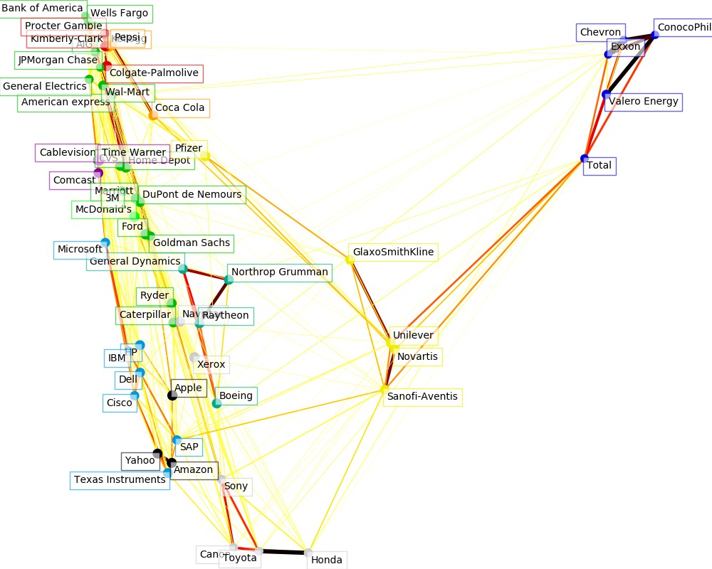
可視化
將3個模型的輸出組合成2D圖,其中節點表示股票符號(Symbol):
- 聚類標記,用於定義節點的顏色
- 稀疏協方差模型,用於顯示邊的強度
- 2D嵌入,用於定位節點
此示例包含大量可視化相關的代碼,挑戰之一是如何放置標簽以最大程度地減少重疊。為此,我們使用基於每個軸上最近鄰居的方向的啟發式方法。
代碼實現[Python]
# -*- coding: utf-8 -*-

# Author: Gael Varoquaux gael.varoquaux@normalesup.org
# License: BSD 3 clause

import sys

import numpy as np
import matplotlib.pyplot as plt
from matplotlib.collections import LineCollection

import pandas as pd

from sklearn import cluster, covariance, manifold

print(__doc__)


# #############################################################################
# 從Internet上獲取股票數據

# The data is from 2003 - 2008. This is reasonably calm: (not too long ago so
# that we get high-tech firms, and before the 2008 crash). This kind of
# historical data can be obtained for from APIs like the quandl.com and
# alphavantage.co ones.

symbol_dict = {
    'TOT': 'Total',
    'XOM': 'Exxon',
    'CVX': 'Chevron',
    'COP': 'ConocoPhillips',
    'VLO': 'Valero Energy',
    'MSFT': 'Microsoft',
    'IBM': 'IBM',
    'TWX': 'Time Warner',
    'CMCSA': 'Comcast',
    'CVC': 'Cablevision',
    'YHOO': 'Yahoo',
    'DELL': 'Dell',
    'HPQ': 'HP',
    'AMZN': 'Amazon',
    'TM': 'Toyota',
    'CAJ': 'Canon',
    'SNE': 'Sony',
    'F': 'Ford',
    'HMC': 'Honda',
    'NAV': 'Navistar',
    'NOC': 'Northrop Grumman',
    'BA': 'Boeing',
    'KO': 'Coca Cola',
    'MMM': '3M',
    'MCD': 'McDonald\'s',
    'PEP': 'Pepsi',
    'K': 'Kellogg',
    'UN': 'Unilever',
    'MAR': 'Marriott',
    'PG': 'Procter Gamble',
    'CL': 'Colgate-Palmolive',
    'GE': 'General Electrics',
    'WFC': 'Wells Fargo',
    'JPM': 'JPMorgan Chase',
    'AIG': 'AIG',
    'AXP': 'American express',
    'BAC': 'Bank of America',
    'GS': 'Goldman Sachs',
    'AAPL': 'Apple',
    'SAP': 'SAP',
    'CSCO': 'Cisco',
    'TXN': 'Texas Instruments',
    'XRX': 'Xerox',
    'WMT': 'Wal-Mart',
    'HD': 'Home Depot',
    'GSK': 'GlaxoSmithKline',
    'PFE': 'Pfizer',
    'SNY': 'Sanofi-Aventis',
    'NVS': 'Novartis',
    'KMB': 'Kimberly-Clark',
    'R': 'Ryder',
    'GD': 'General Dynamics',
    'RTN': 'Raytheon',
    'CVS': 'CVS',
    'CAT': 'Caterpillar',
    'DD': 'DuPont de Nemours'}


symbols, names = np.array(sorted(symbol_dict.items())).T

quotes = []

for symbol in symbols:
    print('Fetching quote history for %r' % symbol, file=sys.stderr)
    url = ('https://raw.githubusercontent.com/scikit-learn/examples-data/'
           'master/financial-data/{}.csv')
    quotes.append(pd.read_csv(url.format(symbol)))

close_prices = np.vstack([q['close'] for q in quotes])
open_prices = np.vstack([q['open'] for q in quotes])

# The daily variations of the quotes are what carry most information
variation = close_prices - open_prices


# #############################################################################
# 從相關性學習圖結構
edge_model = covariance.GraphicalLassoCV(cv=5)

# standardize the time series: using correlations rather than covariance
# is more efficient for structure recovery
X = variation.copy().T
X /= X.std(axis=0)
edge_model.fit(X)

# #############################################################################
# 親和力傳播聚類

_, labels = cluster.affinity_propagation(edge_model.covariance_)
n_labels = labels.max()

for i in range(n_labels + 1):
    print('Cluster %i: %s' % ((i + 1), ', '.join(names[labels == i])))

# #############################################################################
# 計算低維embedding: find the best position of
# the nodes (the stocks) on a 2D plane

# We use a dense eigen_solver to achieve reproducibility (arpack is
# initiated with random vectors that we don't control). In addition, we
# use a large number of neighbors to capture the large-scale structure.
node_position_model = manifold.LocallyLinearEmbedding(
    n_components=2, eigen_solver='dense', n_neighbors=6)

embedding = node_position_model.fit_transform(X.T).T

# #############################################################################
# 可視化
plt.figure(1, facecolor='w', figsize=(10, 8))
plt.clf()
ax = plt.axes([0., 0., 1., 1.])
plt.axis('off')

# Display a graph of the partial correlations
partial_correlations = edge_model.precision_.copy()
d = 1 / np.sqrt(np.diag(partial_correlations))
partial_correlations *= d
partial_correlations *= d[:, np.newaxis]
non_zero = (np.abs(np.triu(partial_correlations, k=1)) > 0.02)

# Plot the nodes using the coordinates of our embedding
plt.scatter(embedding[0], embedding[1], s=100 * d ** 2, c=labels,
            cmap=plt.cm.nipy_spectral)

# Plot the edges
start_idx, end_idx = np.where(non_zero)
# a sequence of (*line0*, *line1*, *line2*), where::
#            linen = (x0, y0), (x1, y1), ... (xm, ym)
segments = [[embedding[:, start], embedding[:, stop]]
            for start, stop in zip(start_idx, end_idx)]
values = np.abs(partial_correlations[non_zero])
lc = LineCollection(segments,
                    zorder=0, cmap=plt.cm.hot_r,
                    norm=plt.Normalize(0, .7 * values.max()))
lc.set_array(values)
lc.set_linewidths(15 * values)
ax.add_collection(lc)

# Add a label to each node. The challenge here is that we want to
# position the labels to avoid overlap with other labels
for index, (name, label, (x, y)) in enumerate(
        zip(names, labels, embedding.T)):

    dx = x - embedding[0]
    dx[index] = 1
    dy = y - embedding[1]
    dy[index] = 1
    this_dx = dx[np.argmin(np.abs(dy))]
    this_dy = dy[np.argmin(np.abs(dx))]
    if this_dx > 0:
        horizontalalignment = 'left'
        x = x + .002
    else:
        horizontalalignment = 'right'
        x = x - .002
    if this_dy > 0:
        verticalalignment = 'bottom'
        y = y + .002
    else:
        verticalalignment = 'top'
        y = y - .002
    plt.text(x, y, name, size=10,
             horizontalalignment=horizontalalignment,
             verticalalignment=verticalalignment,
             bbox=dict(facecolor='w',
                       edgecolor=plt.cm.nipy_spectral(label / float(n_labels)),
                       alpha=.6))

plt.xlim(embedding[0].min() - .15 * embedding[0].ptp(),
         embedding[0].max() + .10 * embedding[0].ptp(),)
plt.ylim(embedding[1].min() - .03 * embedding[1].ptp(),
         embedding[1].max() + .03 * embedding[1].ptp())

plt.show()
代碼執行
代碼運行時間大約:0分4.857秒。
運行代碼輸出的文本內容如下:
Cluster 1: Apple, Amazon, Yahoo
Cluster 2: Comcast, Cablevision, Time Warner
Cluster 3: ConocoPhillips, Chevron, Total, Valero Energy, Exxon
Cluster 4: Cisco, Dell, HP, IBM, Microsoft, SAP, Texas Instruments
Cluster 5: Boeing, General Dynamics, Northrop Grumman, Raytheon
Cluster 6: AIG, American express, Bank of America, Caterpillar, CVS, DuPont de Nemours, Ford, General Electrics, Goldman Sachs, Home Depot, JPMorgan Chase, Marriott, 3M, Ryder, Wells Fargo, Wal-Mart
Cluster 7: McDonald's
Cluster 8: GlaxoSmithKline, Novartis, Pfizer, Sanofi-Aventis, Unilever
Cluster 9: Kellogg, Coca Cola, Pepsi
Cluster 10: Colgate-Palmolive, Kimberly-Clark, Procter Gamble
Cluster 11: Canon, Honda, Navistar, Sony, Toyota, Xerox
運行代碼輸出的圖片內容如下:
源碼下載
- Python版源碼文件: plot_stock_market.py
- Jupyter Notebook版源碼文件: plot_stock_market.ipynb