Tidy 总结了有关模型组件的信息。模型组件可能是回归中的单个项、单个假设、聚类或类。 tidy 所认为的模型组件的确切含义因模型而异,但通常是不言而喻的。如果模型具有多种不同类型的组件,您将需要指定要返回哪些组件。
参数
- x
-
从
gmm::gmm()返回的gmm对象。 - conf.int
-
逻辑指示是否在整理的输出中包含置信区间。默认为
FALSE。 - conf.level
-
用于置信区间的置信水平(如果
conf.int = TRUE)。必须严格大于 0 且小于 1。默认为 0.95,对应于 95% 的置信区间。 - exponentiate
-
逻辑指示是否对系数估计值取幂。这对于逻辑回归和多项回归来说是典型的,但如果没有 log 或 logit 链接,那么这是一个坏主意。默认为
FALSE。 - ...
-
附加参数。不曾用过。仅需要匹配通用签名。注意:拼写错误的参数将被吸收到
...中,并被忽略。如果拼写错误的参数有默认值,则将使用默认值。例如,如果您传递conf.lvel = 0.9,所有计算将使用conf.level = 0.95进行。这里有两个异常:
也可以看看
其他 gmm 整理器:glance.gmm()
值
带有列的 tibble::tibble():
- conf.high
-
估计置信区间的上限。
- conf.low
-
估计置信区间的下限。
- estimate
-
回归项的估计值。
- p.value
-
与观察到的统计量相关的两侧 p 值。
- statistic
-
在回归项非零的假设中使用的 T-statistic 的值。
- std.error
-
回归项的标准误差。
- term
-
回归项的名称。
例子
# load libraries for models and data
library(gmm)
# examples come from the "gmm" package
# CAPM test with GMM
data(Finance)
r <- Finance[1:300, 1:10]
rm <- Finance[1:300, "rm"]
rf <- Finance[1:300, "rf"]
z <- as.matrix(r - rf)
t <- nrow(z)
zm <- rm - rf
h <- matrix(zm, t, 1)
res <- gmm(z ~ zm, x = h)
# tidy result
tidy(res)
#> # A tibble: 20 × 5
#> term estimate std.error statistic p.value
#> <chr> <dbl> <dbl> <dbl> <dbl>
#> 1 WMK_(Intercept) -0.00467 0.0566 -0.0824 9.34e- 1
#> 2 UIS_(Intercept) 0.102 0.126 0.816 4.15e- 1
#> 3 ORB_(Intercept) 0.146 0.203 0.718 4.73e- 1
#> 4 MAT_(Intercept) 0.0359 0.110 0.326 7.45e- 1
#> 5 ABAX_(Intercept) 0.0917 0.288 0.318 7.50e- 1
#> 6 T_(Intercept) 0.0231 0.0774 0.298 7.65e- 1
#> 7 EMR_(Intercept) 0.0299 0.0552 0.542 5.88e- 1
#> 8 JCS_(Intercept) 0.117 0.155 0.756 4.50e- 1
#> 9 VOXX_(Intercept) 0.0209 0.182 0.115 9.09e- 1
#> 10 ZOOM_(Intercept) -0.219 0.202 -1.08 2.79e- 1
#> 11 WMK_zm 0.317 0.126 2.52 1.16e- 2
#> 12 UIS_zm 1.26 0.230 5.49 3.94e- 8
#> 13 ORB_zm 1.49 0.428 3.49 4.87e- 4
#> 14 MAT_zm 1.01 0.218 4.66 3.09e- 6
#> 15 ABAX_zm 1.09 0.579 1.88 5.98e- 2
#> 16 T_zm 0.849 0.154 5.52 3.41e- 8
#> 17 EMR_zm 0.741 0.0998 7.43 1.13e-13
#> 18 JCS_zm 0.959 0.348 2.76 5.85e- 3
#> 19 VOXX_zm 1.48 0.369 4.01 6.04e- 5
#> 20 ZOOM_zm 2.08 0.321 6.46 1.02e-10
tidy(res, conf.int = TRUE)
#> # A tibble: 20 × 7
#> term estimate std.error statistic p.value conf.low conf.high
#> <chr> <dbl> <dbl> <dbl> <dbl> <dbl> <dbl>
#> 1 WMK_(Intercep… -0.00467 0.0566 -0.0824 9.34e- 1 -0.116 0.106
#> 2 UIS_(Intercep… 0.102 0.126 0.816 4.15e- 1 -0.144 0.348
#> 3 ORB_(Intercep… 0.146 0.203 0.718 4.73e- 1 -0.252 0.544
#> 4 MAT_(Intercep… 0.0359 0.110 0.326 7.45e- 1 -0.180 0.252
#> 5 ABAX_(Interce… 0.0917 0.288 0.318 7.50e- 1 -0.473 0.656
#> 6 T_(Intercept) 0.0231 0.0774 0.298 7.65e- 1 -0.129 0.175
#> 7 EMR_(Intercep… 0.0299 0.0552 0.542 5.88e- 1 -0.0782 0.138
#> 8 JCS_(Intercep… 0.117 0.155 0.756 4.50e- 1 -0.186 0.420
#> 9 VOXX_(Interce… 0.0209 0.182 0.115 9.09e- 1 -0.335 0.377
#> 10 ZOOM_(Interce… -0.219 0.202 -1.08 2.79e- 1 -0.616 0.177
#> 11 WMK_zm 0.317 0.126 2.52 1.16e- 2 0.0708 0.564
#> 12 UIS_zm 1.26 0.230 5.49 3.94e- 8 0.812 1.71
#> 13 ORB_zm 1.49 0.428 3.49 4.87e- 4 0.654 2.33
#> 14 MAT_zm 1.01 0.218 4.66 3.09e- 6 0.588 1.44
#> 15 ABAX_zm 1.09 0.579 1.88 5.98e- 2 -0.0451 2.22
#> 16 T_zm 0.849 0.154 5.52 3.41e- 8 0.547 1.15
#> 17 EMR_zm 0.741 0.0998 7.43 1.13e-13 0.545 0.936
#> 18 JCS_zm 0.959 0.348 2.76 5.85e- 3 0.277 1.64
#> 19 VOXX_zm 1.48 0.369 4.01 6.04e- 5 0.758 2.21
#> 20 ZOOM_zm 2.08 0.321 6.46 1.02e-10 1.45 2.71
tidy(res, conf.int = TRUE, conf.level = .99)
#> # A tibble: 20 × 7
#> term estimate std.error statistic p.value conf.low conf.high
#> <chr> <dbl> <dbl> <dbl> <dbl> <dbl> <dbl>
#> 1 WMK_(Intercep… -0.00467 0.0566 -0.0824 9.34e- 1 -0.151 0.141
#> 2 UIS_(Intercep… 0.102 0.126 0.816 4.15e- 1 -0.221 0.426
#> 3 ORB_(Intercep… 0.146 0.203 0.718 4.73e- 1 -0.377 0.669
#> 4 MAT_(Intercep… 0.0359 0.110 0.326 7.45e- 1 -0.248 0.320
#> 5 ABAX_(Interce… 0.0917 0.288 0.318 7.50e- 1 -0.650 0.834
#> 6 T_(Intercept) 0.0231 0.0774 0.298 7.65e- 1 -0.176 0.223
#> 7 EMR_(Intercep… 0.0299 0.0552 0.542 5.88e- 1 -0.112 0.172
#> 8 JCS_(Intercep… 0.117 0.155 0.756 4.50e- 1 -0.281 0.515
#> 9 VOXX_(Interce… 0.0209 0.182 0.115 9.09e- 1 -0.447 0.489
#> 10 ZOOM_(Interce… -0.219 0.202 -1.08 2.79e- 1 -0.740 0.302
#> 11 WMK_zm 0.317 0.126 2.52 1.16e- 2 -0.00656 0.641
#> 12 UIS_zm 1.26 0.230 5.49 3.94e- 8 0.671 1.85
#> 13 ORB_zm 1.49 0.428 3.49 4.87e- 4 0.391 2.60
#> 14 MAT_zm 1.01 0.218 4.66 3.09e- 6 0.454 1.58
#> 15 ABAX_zm 1.09 0.579 1.88 5.98e- 2 -0.401 2.58
#> 16 T_zm 0.849 0.154 5.52 3.41e- 8 0.453 1.25
#> 17 EMR_zm 0.741 0.0998 7.43 1.13e-13 0.484 0.998
#> 18 JCS_zm 0.959 0.348 2.76 5.85e- 3 0.0627 1.85
#> 19 VOXX_zm 1.48 0.369 4.01 6.04e- 5 0.530 2.43
#> 20 ZOOM_zm 2.08 0.321 6.46 1.02e-10 1.25 2.91
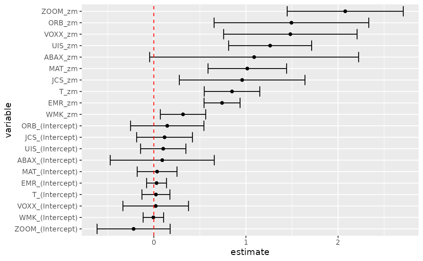
# coefficient plot
library(ggplot2)
library(dplyr)
tidy(res, conf.int = TRUE) %>%
mutate(variable = reorder(term, estimate)) %>%
ggplot(aes(estimate, variable)) +
geom_point() +
geom_errorbarh(aes(xmin = conf.low, xmax = conf.high)) +
geom_vline(xintercept = 0, color = "red", lty = 2)
 # from a function instead of a matrix
g <- function(theta, x) {
e <- x[, 2:11] - theta[1] - (x[, 1] - theta[1]) %*% matrix(theta[2:11], 1, 10)
gmat <- cbind(e, e * c(x[, 1]))
return(gmat)
}
x <- as.matrix(cbind(rm, r))
res_black <- gmm(g, x = x, t0 = rep(0, 11))
tidy(res_black)
#> # A tibble: 11 × 5
#> term estimate std.error statistic p.value
#> <chr> <dbl> <dbl> <dbl> <dbl>
#> 1 Theta[1] 0.516 0.172 3.00 2.72e- 3
#> 2 Theta[2] 1.12 0.116 9.65 5.02e-22
#> 3 Theta[3] 0.680 0.197 3.45 5.65e- 4
#> 4 Theta[4] -0.0322 0.424 -0.0761 9.39e- 1
#> 5 Theta[5] 0.850 0.155 5.49 4.05e- 8
#> 6 Theta[6] -0.205 0.479 -0.429 6.68e- 1
#> 7 Theta[7] 0.625 0.122 5.14 2.73e- 7
#> 8 Theta[8] 1.05 0.0687 15.3 5.03e-53
#> 9 Theta[9] 0.640 0.233 2.75 5.92e- 3
#> 10 Theta[10] 0.596 0.295 2.02 4.36e- 2
#> 11 Theta[11] 1.16 0.240 4.82 1.45e- 6
tidy(res_black, conf.int = TRUE)
#> # A tibble: 11 × 7
#> term estimate std.error statistic p.value conf.low conf.high
#> <chr> <dbl> <dbl> <dbl> <dbl> <dbl> <dbl>
#> 1 Theta[1] 0.516 0.172 3.00 2.72e- 3 0.178 0.853
#> 2 Theta[2] 1.12 0.116 9.65 5.02e-22 0.889 1.34
#> 3 Theta[3] 0.680 0.197 3.45 5.65e- 4 0.293 1.07
#> 4 Theta[4] -0.0322 0.424 -0.0761 9.39e- 1 -0.862 0.798
#> 5 Theta[5] 0.850 0.155 5.49 4.05e- 8 0.546 1.15
#> 6 Theta[6] -0.205 0.479 -0.429 6.68e- 1 -1.14 0.733
#> 7 Theta[7] 0.625 0.122 5.14 2.73e- 7 0.387 0.864
#> 8 Theta[8] 1.05 0.0687 15.3 5.03e-53 0.919 1.19
#> 9 Theta[9] 0.640 0.233 2.75 5.92e- 3 0.184 1.10
#> 10 Theta[10] 0.596 0.295 2.02 4.36e- 2 0.0171 1.17
#> 11 Theta[11] 1.16 0.240 4.82 1.45e- 6 0.686 1.63
# APT test with Fama-French factors and GMM
f1 <- zm
f2 <- Finance[1:300, "hml"] - rf
f3 <- Finance[1:300, "smb"] - rf
h <- cbind(f1, f2, f3)
res2 <- gmm(z ~ f1 + f2 + f3, x = h)
td2 <- tidy(res2, conf.int = TRUE)
td2
#> # A tibble: 40 × 7
#> term estimate std.error statistic p.value conf.low conf.high
#> <chr> <dbl> <dbl> <dbl> <dbl> <dbl> <dbl>
#> 1 WMK_(Intercept) -0.0240 0.0548 -0.438 0.662 -0.131 0.0834
#> 2 UIS_(Intercept) 0.0723 0.127 0.567 0.570 -0.177 0.322
#> 3 ORB_(Intercept) 0.114 0.212 0.534 0.593 -0.303 0.530
#> 4 MAT_(Intercept) 0.0694 0.0979 0.709 0.478 -0.122 0.261
#> 5 ABAX_(Intercep… 0.0668 0.275 0.242 0.808 -0.473 0.606
#> 6 T_(Intercept) 0.0195 0.0745 0.262 0.793 -0.126 0.165
#> 7 EMR_(Intercept) 0.0217 0.0538 0.404 0.687 -0.0837 0.127
#> 8 JCS_(Intercept) 0.0904 0.154 0.586 0.558 -0.212 0.393
#> 9 VOXX_(Intercep… -0.00706 0.179 -0.0394 0.969 -0.359 0.344
#> 10 ZOOM_(Intercep… -0.189 0.215 -0.878 0.380 -0.610 0.233
#> # ℹ 30 more rows
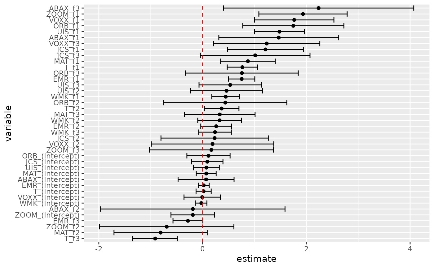
# coefficient plot
td2 %>%
mutate(variable = reorder(term, estimate)) %>%
ggplot(aes(estimate, variable)) +
geom_point() +
geom_errorbarh(aes(xmin = conf.low, xmax = conf.high)) +
geom_vline(xintercept = 0, color = "red", lty = 2)
# from a function instead of a matrix
g <- function(theta, x) {
e <- x[, 2:11] - theta[1] - (x[, 1] - theta[1]) %*% matrix(theta[2:11], 1, 10)
gmat <- cbind(e, e * c(x[, 1]))
return(gmat)
}
x <- as.matrix(cbind(rm, r))
res_black <- gmm(g, x = x, t0 = rep(0, 11))
tidy(res_black)
#> # A tibble: 11 × 5
#> term estimate std.error statistic p.value
#> <chr> <dbl> <dbl> <dbl> <dbl>
#> 1 Theta[1] 0.516 0.172 3.00 2.72e- 3
#> 2 Theta[2] 1.12 0.116 9.65 5.02e-22
#> 3 Theta[3] 0.680 0.197 3.45 5.65e- 4
#> 4 Theta[4] -0.0322 0.424 -0.0761 9.39e- 1
#> 5 Theta[5] 0.850 0.155 5.49 4.05e- 8
#> 6 Theta[6] -0.205 0.479 -0.429 6.68e- 1
#> 7 Theta[7] 0.625 0.122 5.14 2.73e- 7
#> 8 Theta[8] 1.05 0.0687 15.3 5.03e-53
#> 9 Theta[9] 0.640 0.233 2.75 5.92e- 3
#> 10 Theta[10] 0.596 0.295 2.02 4.36e- 2
#> 11 Theta[11] 1.16 0.240 4.82 1.45e- 6
tidy(res_black, conf.int = TRUE)
#> # A tibble: 11 × 7
#> term estimate std.error statistic p.value conf.low conf.high
#> <chr> <dbl> <dbl> <dbl> <dbl> <dbl> <dbl>
#> 1 Theta[1] 0.516 0.172 3.00 2.72e- 3 0.178 0.853
#> 2 Theta[2] 1.12 0.116 9.65 5.02e-22 0.889 1.34
#> 3 Theta[3] 0.680 0.197 3.45 5.65e- 4 0.293 1.07
#> 4 Theta[4] -0.0322 0.424 -0.0761 9.39e- 1 -0.862 0.798
#> 5 Theta[5] 0.850 0.155 5.49 4.05e- 8 0.546 1.15
#> 6 Theta[6] -0.205 0.479 -0.429 6.68e- 1 -1.14 0.733
#> 7 Theta[7] 0.625 0.122 5.14 2.73e- 7 0.387 0.864
#> 8 Theta[8] 1.05 0.0687 15.3 5.03e-53 0.919 1.19
#> 9 Theta[9] 0.640 0.233 2.75 5.92e- 3 0.184 1.10
#> 10 Theta[10] 0.596 0.295 2.02 4.36e- 2 0.0171 1.17
#> 11 Theta[11] 1.16 0.240 4.82 1.45e- 6 0.686 1.63
# APT test with Fama-French factors and GMM
f1 <- zm
f2 <- Finance[1:300, "hml"] - rf
f3 <- Finance[1:300, "smb"] - rf
h <- cbind(f1, f2, f3)
res2 <- gmm(z ~ f1 + f2 + f3, x = h)
td2 <- tidy(res2, conf.int = TRUE)
td2
#> # A tibble: 40 × 7
#> term estimate std.error statistic p.value conf.low conf.high
#> <chr> <dbl> <dbl> <dbl> <dbl> <dbl> <dbl>
#> 1 WMK_(Intercept) -0.0240 0.0548 -0.438 0.662 -0.131 0.0834
#> 2 UIS_(Intercept) 0.0723 0.127 0.567 0.570 -0.177 0.322
#> 3 ORB_(Intercept) 0.114 0.212 0.534 0.593 -0.303 0.530
#> 4 MAT_(Intercept) 0.0694 0.0979 0.709 0.478 -0.122 0.261
#> 5 ABAX_(Intercep… 0.0668 0.275 0.242 0.808 -0.473 0.606
#> 6 T_(Intercept) 0.0195 0.0745 0.262 0.793 -0.126 0.165
#> 7 EMR_(Intercept) 0.0217 0.0538 0.404 0.687 -0.0837 0.127
#> 8 JCS_(Intercept) 0.0904 0.154 0.586 0.558 -0.212 0.393
#> 9 VOXX_(Intercep… -0.00706 0.179 -0.0394 0.969 -0.359 0.344
#> 10 ZOOM_(Intercep… -0.189 0.215 -0.878 0.380 -0.610 0.233
#> # ℹ 30 more rows
# coefficient plot
td2 %>%
mutate(variable = reorder(term, estimate)) %>%
ggplot(aes(estimate, variable)) +
geom_point() +
geom_errorbarh(aes(xmin = conf.low, xmax = conf.high)) +
geom_vline(xintercept = 0, color = "red", lty = 2)
相关用法
- R broom tidy.garch 整理 a(n) garch 对象
- R broom tidy.glmnet 整理 a(n) glmnet 对象
- R broom tidy.geeglm 整理 a(n) geeglm 对象
- R broom tidy.glmRob 整理 a(n) glmRob 对象
- R broom tidy.gam 整理 a(n) gam 对象
- R broom tidy.glht 整理 a(n) glht 对象
- R broom tidy.robustbase.glmrob 整理 a(n) glmrob 对象
- R broom tidy.acf 整理 a(n) acf 对象
- R broom tidy.robustbase.lmrob 整理 a(n) lmrob 对象
- R broom tidy.biglm 整理 a(n) biglm 对象
- R broom tidy.rq 整理 a(n) rq 对象
- R broom tidy.kmeans 整理 a(n) kmeans 对象
- R broom tidy.betamfx 整理 a(n) betamfx 对象
- R broom tidy.anova 整理 a(n) anova 对象
- R broom tidy.btergm 整理 a(n) btergm 对象
- R broom tidy.cv.glmnet 整理 a(n) cv.glmnet 对象
- R broom tidy.roc 整理 a(n) roc 对象
- R broom tidy.poLCA 整理 a(n) poLCA 对象
- R broom tidy.emmGrid 整理 a(n) emmGrid 对象
- R broom tidy.Kendall 整理 a(n) Kendall 对象
- R broom tidy.survreg 整理 a(n) survreg 对象
- R broom tidy.ergm 整理 a(n) ergm 对象
- R broom tidy.pairwise.htest 整理 a(n)pairwise.htest 对象
- R broom tidy.coeftest 整理 a(n) coeftest 对象
- R broom tidy.polr 整理 a(n) polr 对象
注:本文由纯净天空筛选整理自等大神的英文原创作品 Tidy a(n) gmm object。非经特殊声明,原始代码版权归原作者所有,本译文未经允许或授权,请勿转载或复制。