本文简要介绍 python 语言中 scipy.cluster.hierarchy.linkage 的用法。
用法:
scipy.cluster.hierarchy.linkage(y, method='single', metric='euclidean', optimal_ordering=False)#执行分层/凝聚聚类。
输入 y 可以是一维压缩距离矩阵或二维观察向量数组。
如果 y 是一维压缩距离矩阵,则 y 必须是 大小的向量,其中 n 是在距离矩阵中配对的原始观测值的数量。此函数的行为与 MATLAB 链接函数非常相似。
返回一个 x 4 矩阵
Z。在 -th 迭代中,具有索引Z[i, 0]和Z[i, 1]的集群组合形成集群 。索引小于 的集群对应于 原始观测值之一。簇Z[i, 0]和Z[i, 1]之间的距离由Z[i, 2]给出。第四个值Z[i, 3]表示新形成的聚类中原始观测值的数量。以下链接方法用于计算两个簇 和 之间的距离 。该算法从尚未在正在形成的层次结构中使用的集群森林开始。当来自该林的两个集群 和 组合成一个集群时, 、 和 将从森林中删除,并将 添加到森林中。当森林中只剩下一个簇时,算法停止,这个簇成为根。
每次迭代都维护一个距离矩阵。
d[i,j]条目对应于原始森林中簇 和 之间的距离。在每次迭代中,算法必须更新距离矩阵以反映新形成的集群 u 与森林中剩余集群的距离。
假设在集群 中有 原始观测值 ,在集群 中有 原始对象 。回想一下, 和 组合在一起形成集群 。让 是林中不是 的任何剩余集群。
以下是计算新形成的簇 和每个 之间距离的方法。
method=’single’ assigns
for all points in cluster and in cluster . This is also known as the Nearest Point Algorithm.
method=’complete’ assigns
for all points in cluster u and in cluster . This is also known by the Farthest Point Algorithm or Voor Hees Algorithm.
method=’average’ assigns
for all points and where and are the cardinalities of clusters and , respectively. This is also called the UPGMA algorithm.
method=’weighted’ assigns
where cluster u was formed with cluster s and t and v is a remaining cluster in the forest (also called WPGMA).
method=’centroid’ assigns
where and are the centroids of clusters and , respectively. When two clusters and are combined into a new cluster , the new centroid is computed over all the original objects in clusters and . The distance then becomes the Euclidean distance between the centroid of and the centroid of a remaining cluster in the forest. This is also known as the UPGMC algorithm.
method=’median’ assigns like the
centroidmethod. When two clusters and are combined into a new cluster , the average of centroids s and t give the new centroid . This is also known as the WPGMC algorithm.method=’ward’ uses the Ward variance minimization algorithm. The new entry is computed as follows,
where is the newly joined cluster consisting of clusters and , is an unused cluster in the forest, , and is the cardinality of its argument. This is also known as the incremental algorithm.
警告:选择森林中的最小距离对时,可能有两个或更多对具有相同的最小距离。此实现可以选择与 MATLAB 版本不同的最小值。
- y: ndarray
一个压缩的距离矩阵。压缩距离矩阵是包含距离矩阵的上三角形的平面阵列。这是
pdist返回的形式。或者, 维度中的 观察向量的集合可以作为 由 数组传递。压缩距离矩阵的所有元素都必须是有限的,即没有 NaNs 或 infs。- method: str,可选
要使用的链接算法。有关完整说明,请参阅下面的
Linkage Methods部分。- metric: str 或函数,可选
在 y 是观察向量集合的情况下使用的距离度量;否则忽略。有关有效距离度量的列表,请参阅
pdist函数。也可以使用自定义距离函数。- optimal_ordering: 布尔型,可选
如果为 True,则链接矩阵将重新排序,以便连续叶子之间的距离最小。当数据可视化时,这会产生更直观的树结构。默认为 False,因为该算法可能很慢,特别是在大型数据集上 [2]。另请参见
optimal_leaf_ordering函数。
- Z: ndarray
层次聚类编码为链接矩阵。
参数 ::
返回 ::
注意:
对于方法‘single’,实现了基于最小生成树的优化算法。它的时间复杂度为。对于方法‘complete’, ‘average’, ‘weighted’和‘ward’,实现了一种称为nearest-neighbors链的算法。它还具有时间复杂度。对于其他方法,以 时间复杂度实现朴素算法。所有算法都使用 内存。有关算法的详细信息,请参阅[1]。
仅当使用欧几里德成对度量时,方法 ‘centroid’, ‘median’ 和 ‘ward’ 才能正确定义。如果 y 作为预先计算的成对距离传递,则用户有责任确保这些距离实际上是欧几里得距离,否则生成的结果将不正确。
参考:
[1]Daniel Mullner,“现代层次、凝聚聚类算法”,arXiv:1109.2378v1。
[2]Ziv Bar-Joseph、David K. Gifford、Tommi S. Jaakkola,“层次聚类的快速最优叶排序”,2001 年。生物信息学 DOI:10.1093/bioinformatics/17.suppl_1.S22
例子:
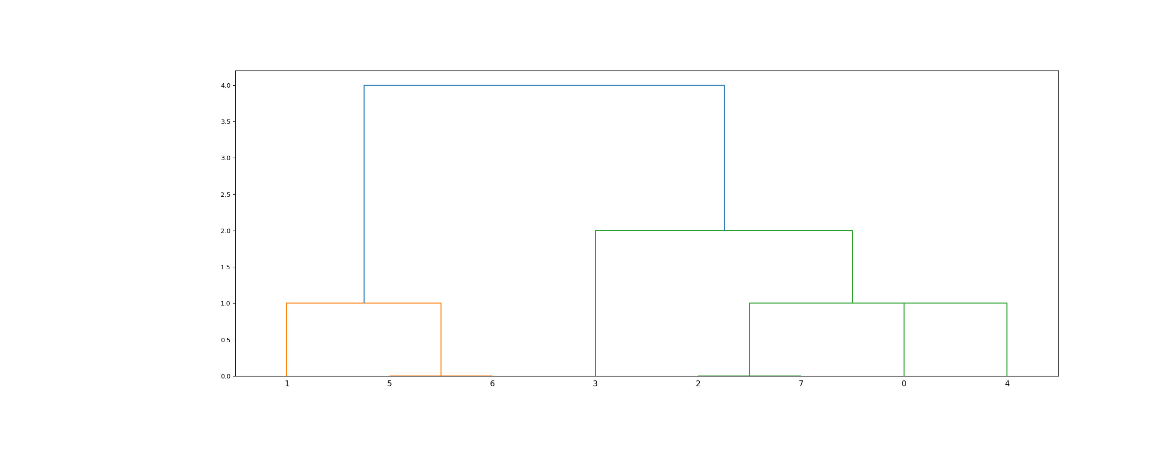
>>> from scipy.cluster.hierarchy import dendrogram, linkage
>>> from matplotlib import pyplot as plt
>>> X = [[i] for i in [2, 8, 0, 4, 1, 9, 9, 0]]
>>> Z = linkage(X, 'ward') >>> fig = plt.figure(figsize=(25, 10)) >>> dn = dendrogram(Z)>>> Z = linkage(X, 'single') >>> fig = plt.figure(figsize=(25, 10)) >>> dn = dendrogram(Z) >>> plt.show()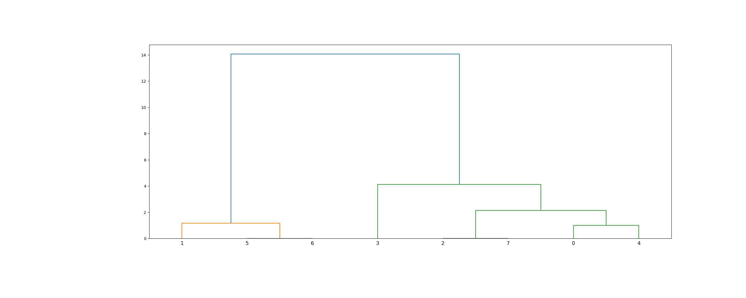
相关用法
- Python SciPy hierarchy.leaves_list用法及代码示例
- Python SciPy hierarchy.leaders用法及代码示例
- Python SciPy hierarchy.ward用法及代码示例
- Python SciPy hierarchy.maxRstat用法及代码示例
- Python SciPy hierarchy.set_link_color_palette用法及代码示例
- Python SciPy hierarchy.fclusterdata用法及代码示例
- Python SciPy hierarchy.median用法及代码示例
- Python SciPy hierarchy.DisjointSet用法及代码示例
- Python SciPy hierarchy.correspond用法及代码示例
- Python SciPy hierarchy.is_isomorphic用法及代码示例
- Python SciPy hierarchy.optimal_leaf_ordering用法及代码示例
- Python SciPy hierarchy.maxinconsts用法及代码示例
- Python SciPy hierarchy.cut_tree用法及代码示例
- Python SciPy hierarchy.fcluster用法及代码示例
- Python SciPy hierarchy.to_tree用法及代码示例
- Python SciPy hierarchy.average用法及代码示例
- Python SciPy hierarchy.dendrogram用法及代码示例
- Python SciPy hierarchy.num_obs_linkage用法及代码示例
- Python SciPy hierarchy.inconsistent用法及代码示例
- Python SciPy hierarchy.complete用法及代码示例
- Python SciPy hierarchy.maxdists用法及代码示例
- Python SciPy hierarchy.is_valid_im用法及代码示例
- Python SciPy hierarchy.centroid用法及代码示例
- Python SciPy hierarchy.single用法及代码示例
- Python SciPy hierarchy.is_monotonic用法及代码示例
注:本文由纯净天空筛选整理自scipy.org大神的英文原创作品 scipy.cluster.hierarchy.linkage。非经特殊声明,原始代码版权归原作者所有,本译文未经允许或授权,请勿转载或复制。