在Jupyter中可视化TensorFlow Graph图的简单方法？

问题描述

可视化TensorFlow Graph图的官方方法是使用TensorBoard，但有时我只是想在Jupyter中工作时快速浏览一下该图。

有没有一种快速的解决方案，理想情况下基于TensorFlow工具或标准SciPy软件包(如matplotlib)，就能在jupyter notebook中可视化Tensorflow Graph？

最佳答案

TensorFlow 2.0现在通过magic命令(例如%tensorboard --logdir logs/train)在Jupyter中支持TensorBoard。这是教程和示例的链接。

需要先加载扩展名(%load_ext tensorboard.notebook)。

以下是使用图形模式@tf.function和tf.keras(在tensorflow==2.0.0-alpha0中)的使用示例：

1.在TF2中使用图形模式的示例(通过tf.compat.v1.disable_eager_execution())

%load_ext tensorboard.notebook
import tensorflow as tf
tf.compat.v1.disable_eager_execution()
from tensorflow.python.ops.array_ops import placeholder
from tensorflow.python.training.gradient_descent import GradientDescentOptimizer
from tensorflow.python.summary.writer.writer import FileWriter

with tf.name_scope('inputs'):
   x = placeholder(tf.float32, shape=[None, 2], name='x')
   y = placeholder(tf.int32, shape=[None], name='y')

with tf.name_scope('logits'):
   layer = tf.keras.layers.Dense(units=2)
   logits = layer(x)

with tf.name_scope('loss'):
   xentropy = tf.nn.sparse_softmax_cross_entropy_with_logits(labels=y, logits=logits)
   loss_op = tf.reduce_mean(xentropy)

with tf.name_scope('optimizer'):
   optimizer = GradientDescentOptimizer(0.01)
   train_op = optimizer.minimize(loss_op)

FileWriter('logs/train', graph=train_op.graph).close()
%tensorboard --logdir logs/train

2.与上述示例相同，但现在使用@tf.function装饰器进行forward-backward传递，并且不禁用立即执行：

%load_ext tensorboard.notebook
import tensorflow as tf
import numpy as np

logdir = 'logs/'
writer = tf.summary.create_file_writer(logdir)
tf.summary.trace_on(graph=True, profiler=True)

@tf.function
def forward_and_backward(x, y, w, b, lr=tf.constant(0.01)):

    with tf.name_scope('logits'):
        logits = tf.matmul(x, w) + b

    with tf.name_scope('loss'):
        loss_fn = tf.nn.sparse_softmax_cross_entropy_with_logits(
            labels=y, logits=logits)
        reduced = tf.reduce_sum(loss_fn)

    with tf.name_scope('optimizer'):
        grads = tf.gradients(reduced, [w, b])
        _ = [x.assign(x - g*lr) for g, x in zip(grads, [w, b])]
    return reduced

# inputs
x = tf.convert_to_tensor(np.ones([1, 2]), dtype=tf.float32)
y = tf.convert_to_tensor(np.array([1]))
# params
w = tf.Variable(tf.random.normal([2, 2]), dtype=tf.float32)
b = tf.Variable(tf.zeros([1, 2]), dtype=tf.float32)

loss_val = forward_and_backward(x, y, w, b)

with writer.as_default():
    tf.summary.trace_export(
        name='NN',
        step=0,
        profiler_outdir=logdir)

%tensorboard --logdir logs/

3.使用tf.keras API：

%load_ext tensorboard.notebook
import tensorflow as tf
import numpy as np
x_train = [np.ones((1, 2))]
y_train = [np.ones(1)]

model = tf.keras.models.Sequential([tf.keras.layers.Dense(2, input_shape=(2, ))])

model.compile(
    optimizer='sgd',
    loss='sparse_categorical_crossentropy',
    metrics=['accuracy'])

logdir = "logs/"

tensorboard_callback = tf.keras.callbacks.TensorBoard(log_dir=logdir)

model.fit(x_train,
          y_train,
          batch_size=1,
          epochs=1,
          callbacks=[tensorboard_callback])

%tensorboard --logdir logs/

这些示例将在单元格下方生成如下内容：

次佳答案

这是我在某个时候从亚历克斯·莫德文采夫(Alex Mordvintsev)的完美notebook复制的解决方法：

from IPython.display import clear_output, Image, display, HTML
import numpy as np    

def strip_consts(graph_def, max_const_size=32):
    """Strip large constant values from graph_def."""
    strip_def = tf.GraphDef()
    for n0 in graph_def.node:
        n = strip_def.node.add() 
        n.MergeFrom(n0)
        if n.op == 'Const':
            tensor = n.attr['value'].tensor
            size = len(tensor.tensor_content)
            if size > max_const_size:
                tensor.tensor_content = "<stripped %d bytes>"%size
    return strip_def

def show_graph(graph_def, max_const_size=32):
    """Visualize TensorFlow graph."""
    if hasattr(graph_def, 'as_graph_def'):
        graph_def = graph_def.as_graph_def()
    strip_def = strip_consts(graph_def, max_const_size=max_const_size)
    code = """
        <script>
          function load() {{
            document.getElementById("{id}").pbtxt = {data};
          }}
        </script>
        <link rel="import" href="https://tensorboard.appspot.com/tf-graph-basic.build.html" onload=load()>
        <div style="height:600px">
          <tf-graph-basic id="{id}"></tf-graph-basic>
        </div>
    """.format(data=repr(str(strip_def)), id='graph'+str(np.random.rand()))

    iframe = """
        <iframe seamless style="width:1200px;height:620px;border:0" srcdoc="{}"></iframe>
    """.format(code.replace('"', '&quot;'))
    display(HTML(iframe))

然后可视化当前图形

show_graph(tf.get_default_graph().as_graph_def())

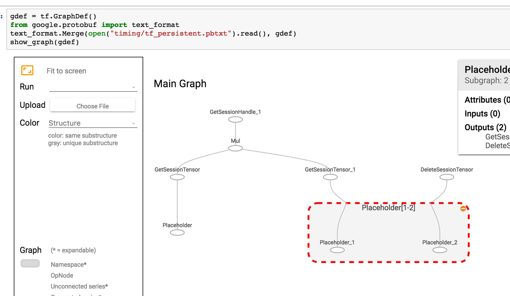
如果您的图形另存为pbtxt，则可以

gdef = tf.GraphDef()
from google.protobuf import text_format
text_format.Merge(open("tf_persistent.pbtxt").read(), gdef)
show_graph(gdef)

你会看到这样的东西

参考资料

• Simple way to visualize a TensorFlow graph in Jupyter?